Chapter 8.4 - Random Forest¶

In Chapter 8.3, we introduced the supervised machine learning classifier called a decision tree. We went through the calculations used to decide split and classification decisions. However, one major limitation of the decision tree is that it is a greedy algorithm. In other words, when the model is making a split decision, that decision is only based on minimizing error in the two resulting subsets (i.e., “local” error minimized). It is possible that a less-ideal split decision at first could lead to a better overall model performance (i.e., “global” error minimized).

Storm Chasing Decision

Consider a situation where you are storm chasing and trying to pick the best supercell towards which to drive your car. Imagine that you are going to use a database of your chasing success / failures to make your decision. One factor might be distance_to_storm, which is how far you are from the ideal viewing location of a storm. Another factor might be storm_environment, which is how supportive the atmosphere is for tornado development around a storm.

You notice that the best decision the majority of the time is to pick the storm closest to you. If you then train your dataset with a decision tree, it might tell you to chase the closest storm! However, when examining the dataset more closely, you notice that the 2nd best choice is storm_environment. In a situation where storm A is 1 mile closer than storm B, but storm B has the better environment, you might instead choose to drive to storm B. This is an example of an interaction between two variables--namely, the influence of distance_to_storm on a chasing decision depends on the storm_environment. This generalization might be obvious to those who storm chase, but it is a big motivating factor for using more complex machine learning models: being farther away from a storm hurts less when the farther storm has a good environment.

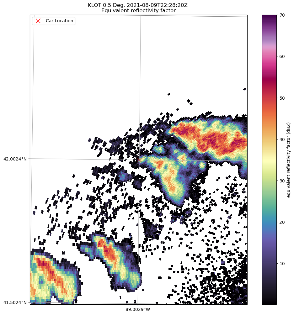
Activity: Consider the situation below, where your car is for some reason dangerously close to the hook echo of a tornadic supercell. What cell would you pick? What is your rationale? Do not share your opinions with anyone yet, but keep track of your opinion.

Now, consider a situation where you have 4 people in the car who always storm chase with eachother and no one else. You randomly assign a subset of storm chase results and factors for each person to examine. Each case could be examined by 1 - 4 people. You then have everyone train a decision tree on their subset and report back with their vote on what storm to chase. To your surpise, you notice that not everyone has the same vote! This is an example of bootstrapping--the process of randomly sampling a dataset (with replacement) and estimating how this modifies the aggregate performance and variability of a decision-making model.

Activity: Take the online survey provided by the instructor.

Chapter 8.4.1 - Decision Tree vs. Random Forest¶

A Random Forest model is comprised of dozens (or thousands) of Decision Trees that each provide a “vote” that gets counted towards the final prediction. If every tree had the same configuration, saw the same data, and calculated split decisions in the same way, these votes (i.e., ensemble prediction) would have very little diversity. The resulting tree ensemble “vote” would not perform much better than a prediction from a single Decision Tree. The strength of the Random Forest approach is that, ideally, an ensemble of Decision Trees trained in slightly different ways on slightly different training data will reduce the high prediction variance of a single Decision Tree. For example, one tree may make a poor splitting decision, while another tree may avoid that split decision because it was trained on different sample data or a different subset of features.

Bagging

Random Forest uses bootstrap aggregating (bagging) to generate an ensemble of slightly different decision trees that: 1) see a smaller sample of the dataset (with replacement); 2) a smaller subset of features (feature bagging; with replacement); and 3) aggregates the predictions of the “weak learners” (i.e., Decision Tree) into a final prediction.

1. Bootstrapping - Each decision tree in the ensemble is “shown” a sample of the dataset (with replacement) and are only allowed to use a random subset of features.

2. Aggregating - The majority of predictions (categorical) or the mean of the predictions (regression) are used to generate the final prediction.

The following example shows the bagging process, where the original dataset (top circles) get sampled for each “weak” learner (boostrapping). The predictions from each learner are aggregated for the final prediction.

Chapter 8.4.2 - Random Forest vs. Weather Model Ensembles¶

The GEFS (Global Ensemble Forecasting System creates ensemble forecasts by providing slightly different initial conditions within an envelope of observational uncertainty. This is somewhat similar to how Random Forest uses bootstrapping to show different ensemble members different data. For example, here are the individual ensemble predictions from the CoD website for the supercell composite parameter:

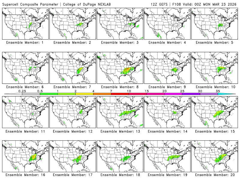
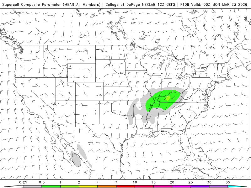
Each ensemble member produces slightly different solutions due to model deficiencies, uncertainty in initial conditions, and the chaotic nature of the atmosphere. When you then calculate the ensemble mean, you are aggregating those predictions. This mean captures the central tendency / signal in the ensemble members and may provide a more realistic prediction. So in a way, you may have already extensively used a product analogous to bagging.

Activity: Assess the mean prediction below. Do you think that it is indicative of the actual risk? What are some characteristics of the ensemble members that might introduce bias into the mean?

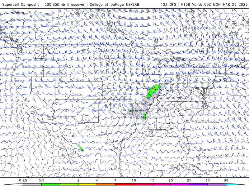
Activity: Assess the deterministic prediction from GFS (Global Forecast System) for the same time period. What is your interpretation of the strength of this prediction? What would you tell someone about the potential for severe weather?

Chapter 8.4.3 - RandomForestClassifier¶

The scikit-learn package has a built-in Random Forest model called RandomForestClassifier. It shares a very similar interface with DecisionTreeClassifier.

The setup for the model is essentially the same.

1. Read in the data

2. Convert the numerical features to numpy arrays

3. Train a RandomForestClassifier with basic settings to make sure it works.

4. Assess the basic model to see how it performs using performance metrics on the testing data:

5. Interrogate a confusion matrix to see if there are issues that need to be addressed:

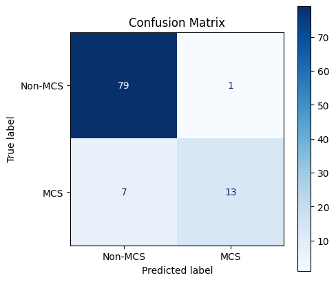
6. If there are large issues, then do model selection using the training and validation datasets.

• Set up the cross validation approach that selects specific training and validation rows.

• For now, use the same parameters we used with DecisionTreeClassifier

7. Use GridSearchCV to find the best random forest model:

8. Assess the best model.

• Your Turn: Did it do better or worse? In what ways?

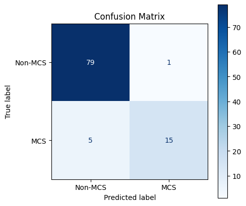
Try some new parameters used by RandomForestClassifier

The RandomForestClassfier has a few extra parameters that might be useful:

1. n_estimators: the number of DecisionTree models included in the ensemble prediction decision.

2. bootstrap: If True, provide each tree with a sample (with replacement). This is True by default.

3. n_jobs: On a multi-core system, you can train individual DecisionTreeClassifier models in parallel. Colab provides 2 cpus, so this number can be 1 or 2. If you are on a different system, you can increase this number.

4. class_weight: If you are experiencing cases where a rare label is not handled well, you can use balanced_subsample to make sure that each bootstrap sample weights certain samples in a way that rewards getting the rare label correct.

Let’s see if modifying n_estimators helps with the performance. I placed n_jobs=2 in the constructor call because that should not influence the model performance, just how fast the model finishes training.

If you used all of the parameters, this one might take awhile, since we are testing over 700 different configurations. Additionally, adding more estimators with n_estimators will make the configurations with 1000 estimators take longer to train.

We will explore Random Forest models more in Lab 8