Chapter 8.3 - Decision Trees¶

A decision tree is a supervised machine learning approach that generates a series of yes/no decisions based on sample features. Ultimately, it uses each learned decision to repeatedly split the samples into two subsets. A hierarchy of many split decisions can produce accurate predictions based on complex interrelationships between variables and labels.

A basic classification decision tree can be described with the following terms:

1. split decision - a rule that separates a dataset into two subsets. For example, testing to see if rain >= 0.01 for a sample would split the dataset into Yes (Rain) and No (No Rain) subsets.

2. Gini impurity - a measure of how homogeneous sample labels are in a subset. The “goal” of the decision tree during each split decision is to make two subsets with homogenous labels.

3. root node - the first rule (split decision).

4. decision nodes - subsequent rules that result in further subset splitting.

5. leaf nodes - classification nodes where no further splits are performed. If the sample labels are not all the same, the most common label is used to classify samples that get to that node.

Chapter 8.3.1 - Gini impurity¶

We can quantify the homogeneity of a set of sample labels by calculating the Gini impurity. In the binary case, this equation is simplified to:

Where $p$ is the fraction of samples in a node with a particular label (e.g., “Yes”), and $1 - p$ is fraction of samples that have the other label (e.g., “No”).

There are some assumptions here:

1. The “observed” label frequencies in a node are assumed to be accurate estimates of the overall (true) label frequencies for the population of samples that may reach this node.

2. To generate a prediction for an “unobserved” sample, we imagine the following randomized rule: select one observed sample at random and use its label as the prediction.

If these assumptions are met, gini impurity measures how likely it is for a split decision to produce an incorrect prediction for a randomly selected sample. The probability comes from both the chance of choosing a sample with, for example, a label of “Yes” or “No” and the chance that you incorrectly predict “Yes” or “No” for that sample.

For a forecasting analogy, imagine grouping historical days by similar atmospheric ingredients. Within one such group, let $p$ be the historical fraction of rainy days. Gini impurity then quantifies how mixed the outcomes are in that ingredient regime: low Gini implies those ingredients almost always lead to the same outcome (high inherent predictability), while high Gini implies substantial overlap between rain and no-rain outcomes (lower inherent predictability).

Examples

If we have 10 samples in a subset and 5 of the samples have a ‘Yes’ label and 5 have a ‘No’ label, the calculation is solved as below:

Example (binary labels): 10 samples total, with 5 Yes and 5 No.

Gini impurity:

As expected, the chance of an incorrect label in this subset is 50% (“coin flip” scenario). The probability of randomly picking a sample with a label of “Yes” is 0.5, and the probability of predicting that sample as a “No” is 0.5. If you remember chained probabilities, the chance of both happening is 0.25. Similarly, the probability of picking a “No” sample label and predicting a “Yes” is 0.25. The additive probability is 0.5 (0.25 + 0.25), because these cases represent mutually exclusive situations where an incorrect prediction is made.

On the other hand, if we had another splitting choice that produced 8 ‘Yes’ labels and 2 ‘No’ labels, the calculation is solved as below:

Example (binary labels): 10 samples total, with 8 Yes and 2 No.

Gini impurity:

This objectively produces a better split decision because the resulting labels are more homogenous. The probability of randomly picking a “Yes” sample label is 0.8, the chance of incorrectly predicting that label is 0.2, and the chance of both happening is 0.16. Similarly, randomly picking a “No” sample label is 0.2, the chance of incorrectly predicting that label is 0.8, and the chance of both happening is 0.16.

Finally, a perfect situation where there are 10 “Yes” sample labels and 0 “No” sample labels:

Example (binary labels): 10 samples total, with 10 Yes and 0 No.

Gini impurity:

Weighted split decisions

The decision tree (specifically CART) calculates the gini impurity for each possible split decision. The final split decision encoded into the model is based on the decision that produces the smallest, weighted gini impurity for both sides of the split decision. Weighted impurity is based on the number of samples on each side of the split. For example, if you had a split decision that produced a subset of 2 samples, which both had “Yes” as a label, and a subset that had 10 samples, of which 5 had “Yes” and 5 had “No” as a label, the weighted Gini impurity would be calculated as:

Split Subset #1

Split Subset #2

Weighted Gini impurity

Your Turn: Consider the two possible split decisions below. Calculate the weighted gini impurity for each case. Which one is the best choice?

Chapter 8.3.2 - Scikit-Learn DecisionTreeClassifier¶

As is the case with all supervised learning techniques, you are required to provide “expert” labels that are associated with each feature vector. Supervised learning techniques use a variety of ways to accurately model relationships between feature vectors and the given labels. As is described above, the decision tree attempts to create accurate predictions by applying a series of split decisions until samples are separated into homogeneous subsets. The idea is that similar cases will cascade down the decision tree nodes along similar paths, eventually ending up in the same final grouping. If the samples used to create (i.e., train) the decision tree are representative of the population, then unobserved/unlabeled samples should also follow these paths in the tree and be assigned accurate predictions.

Scikit-Learn has a decision tree model called DecisionTreeClassifier. This model uses the algorithm described above (or similar) to create split decision rules for the root node and decision nodes, so that sample subsets are ultimately organized into leaf nodes with homogeneous labels. Once in the leaf node, the classification decision is based on the most frequent label in that node.

The decision tree comes with useful default settings, but a few settings you may want to change/tweak are as follows:

• max_depth: This is the count of decision nodes + leaf node beyond the root node. A max_depth of 2 would produce a tree like this:

Other parameters

• min_samples_split: If max_depth is not set, the decision tree will continue to generate splitting rules as long as the subset passed to that node has at least this many samples. For example, if this is set to 2 (default), it will be converted to a leaf node if only one sample is available.

• min_impurity_decrease: A splitting decision will be made, as long as the resulting, weighted impurity is at least this much lower than the impurity in the original subset.

Decision tree properties

• classes_: the ordered labels in the tree.

• feature_importances_: the average decrease in impurity produced by split decsions for each feature. More important features are associated with a larger decrease in impurity on average.

Chapter 8.3.3 - Training a decision tree¶

We will use the storm morphology dataset once again. However, we will simplify the predictions by converting them to:

0: not an MCS
1: an MCS

The process of training the model is very similar to KMeans. We first need to transform the pandas data to numpy using only the numeric columns. You can print out the feature vectors (x_train, x_val, x_test) and labels (y_train, y_val, y_test) to examine their numpy representation.

Next, import the subclass from sklearn.tree and use .fit to train the CART classifier on the training data (x_train and y_train). We will use max_depth=3 to help visualize the tree.

We can use plot_tree on the trained instance to examine its structure.

Activity

Get into groups of two. Interpret the graph below. What does each split decision mean? Can you confirm the Gini impurity scores for the leaf nodes? Can you calculate the following training data metrics and interpret what they mean? The basic decision tree should be deterministic, but check to make sure that this is true if you run it multiple times.

True Positive or TP - Count of correct MCS predictions. In other words, the count of actual MCS labels in a leaf node that has MCS as the prediction

False Positive or FP - Count of incorrect MCS predictions. In other words, the count of actual Non-MCS labels in a leaf node that has MCS as the prediction.

False Negative or FN - Count of how many actual MCS samples are incorrectly labeled as Non-MCS. In other words, the count of actual MCS samples in a leaf node that has Non-MCS as the prediction.

True Negative or TN - Count of how many actual Non-MCS samples are correctly labeled as Non-MCS. In other words, the count of actual Non-MCS samples in a leaf node that has Non-MCS as the prediction.

Accuracy = $\frac{TP + TN}{TP + FN + FP + TN}$

Precision = $\frac{TP}{TP + FP}$

Recall = $\frac{TP}{TP + FN}$

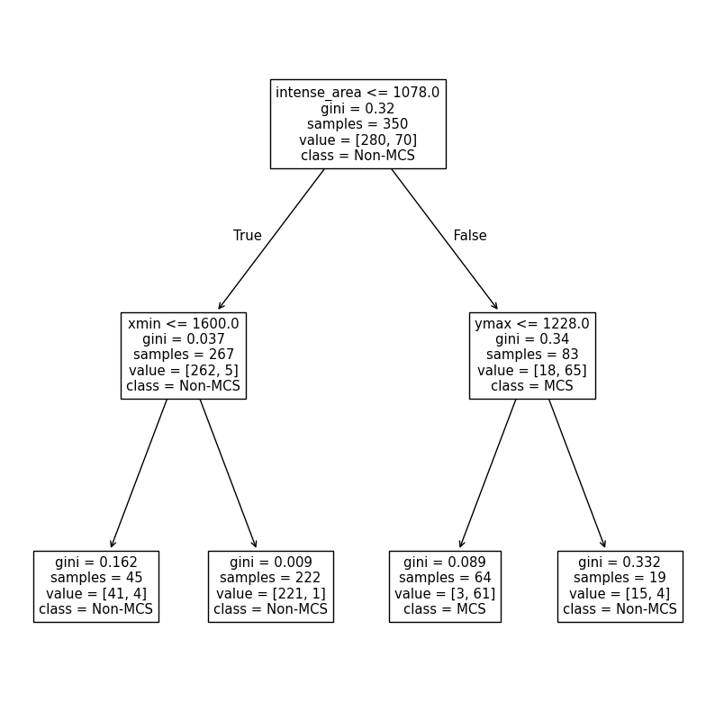
We can create custom functions to calculate the metrics above. At some point, we wil use the built-in functions, but this is a useful exercise to understand how models are assessed.

The DecisionTreeClassifier method named predict takes a numpy array of feature vectors and assigns each vector a label (in this case, 0 for Non-MCS and 1 for MCS).

We have the “ground truth” in y_train, so we can directly compare all of the predictions with y_train to determine the performance of the model. We can perform a comparison to see if the value at each index in y_train_predictions and y_train. For example, if y_train_predictions[0] is True and y_train[0] is True, we know the feature vector at index 0 has a correct prediction. Additionally, since we know True and False are just special cases for int (True is 1, False is 0), we can find the sum of this comparison. This sum is equivalent to how many times the prediction is correct (TP + TN). If we divide this number by the total number of samples, we can get the accuracy.

Activity: Get into groups of 2. Using numpy only, calculate TP, FP, FN, and TN. Using these values, calculate accuracy, precision, and recall. Compare the results to the official sklearn.metrics methods--namely accuracy_score, precision_score, and recall_score. Do they match up? Why might recall and precision be different from accuracy? What does that tell you about model performance on the MCS label? HINT: Think of what conditions must be true in both y_train and y_train_predictions for each case.

Chapter 8.3.4 - Model Selection¶

You may have had this thought in the previous section: “How could I improve the model performance?” I hope you did, at least! Lucky for us, there are several ways we can modify the decision tree to make it work better for our purposes. First, we must consider generalizability when selecting the best performing model. Since we are forbidden from using the testing dataset until the final model performance test, we must use a different dataset. In this case, we will use a predefined validation dataset to simulate what we might encounter in the testing dataset. The best performing model is selected based on maximizing (or minimizing) a particular metric. One very useful metric is the F-score. This score combines both precision and recall into one metric. In addition, it uses the harmonic mean to enforce good performance of both metrics.

For example, the mean of a precision of 0.6 and 0.9 is 0.75, whereas the F-score above would result in 0.72 for a relatively poor precision score. This is to make sure that a prediction of an MCS is accurate and true MCS cases are detected at a high rate. We will use the f1_score from sklearn to find the best performing version of the model on the validation dataset.

One parameter we can change is max_depth. This is useful for limiting overfitting, which is the tendency for models to “memorize” or become too specific to the training dataset. As you can see above, the training results are very good--accuracy of 95% and precision and recall near 90%. However, we expect very good metrics because the model has already seen these data. What about previously unseen data in validation and eventually testing data?

Your turn: Get into a group of 2 and interpret the results from the following experiments that modify max_depth. Look up the documentation of DecisionTreeClassifier and see if there are other parameters you could test to try to improve the performance.

Automated model selection

sklearn has an automated way to test out many different model configurations: GridSearchCV. This class requires you to think about the following options:

1. estimator: this is your untrained DecisionTreeClassifier instance. Do not run fit.

2. param_grid: this is a dictionary with the parameter names and all the possible values you want to test with that parameter.

3. scoring: this defines how GridSearchCV will determine the “best performing” model on validation data.

4. cv: this is how you will separate the training and validation data. In some cases, it might be appropriate to have sklearn handle this with an approach that randomly removes 10% of the data in k different ways. In our case, we will use a predefined split, since it is important to examine “new” data that has temporal independence.

This approach essentially recreates the loops we did in the previous problems. You just have to define the possible values for each parameter.

The first step is to look up the documentation for the model you are using. We are using a DecisionTreeClassifier. On that page you will see Parameters along with several different names of parameters and descriptions. You can try different ranges of numbers that make sense for each parameter. These need to be put in a dictionary.

For this case, we will test the following values to see which combination works best:

1. test criterion of gini (we calculated this earlier) or entropy

2. test max_depth of None (no limit), 2, 4, 6, 8, and 12

3. test min_samples_split of 2, 5, 10, and 20

4. test min_samples_leaf of 1, 2, 5, and 10

We can use ParameterGrid to see all the different combinations.

Answer in the markdown in your own words:

Why are there 192 rows?

Give an example of manually creating a DecisionTreeClassifier model based on the parameters in row 50 (index 49).

Next, we will define the split used to decide what data are supplied to the training process and what data are supplied for the validation process. Since we already have those subsets, we will use the PredefinedSplit approach.

The model selection approach, by default, assumes that we have one subset of feature vector information (i.e., train_x and val_x) as well as one subset of label information (i.e., train_y and val_y).

The best way to combine these two subsets is to use concatenate from numpy. We will use this to “attach” val on to the end of train. As long as we know where this happens, it is easy to define how to tell the model selection step how to split the data.

First, here is a smaller example:

trainx is an ndarray of 2 feature vectors with 3 features and trainy is a ndarray of 2 labels associated with those feature vectors. Similarly, valx and valy are the same, except for one sample.

When you run the concatenate method, you see the result is just a combination of the train and val subsets.

If you wanted to tell the model selection approach that these indices were train with a value of -1 (not in the ‘val’ set) and val with a value of 0 (in the val set), you would define split as you do below. The model selection approach will keep all indices of 0 off to the side and use all indices of -1 to train each model variant. Each model variant will tested with the 0 indices (the validation data), and the best performing model on those data will be selected.

Here is the full concatenation:

We know that the train_x data end at index len(train_x), so we can easily create the -1 and 0 arrays using a number of approaches, for example:

We then pass this array into PredefinedSplit

Finally, we build a basic DecisionTreeClassifier and pass the required information into GridSearchCV. The new code here is:

1. make_scorer: a wrapper around the f1_score we used before.

2. refit: if True, retrain the best performing model and provide it as best_estimator_.

We will practice this further in Lab 7.