%%bash
pip install cartopy > /dev/null
pip install xarray > /dev/null

mkdir storm_mode
cd storm_mode
wget -nc -q https://raw.githubusercontent.com/ahaberlie/unidata-workshop-2018/refs/heads/master/workshop/data/training/sample_train_data.csv
wget -nc -q https://raw.githubusercontent.com/ahaberlie/unidata-workshop-2018/refs/heads/master/workshop/data/training/sample_test_data.csv

Chapter 8.2 - Clustering¶

Clustering (or Cluster Analysis describes a group of unsupervised machine learning techniques. The purpose of these techniques is to organize unlabled samples (and their associated feature vectors) into meaningful groups. Ideal groups will promote within group similarity and between group differences.

There are many clustering algorithms, but in this chapter we will focus on the following:

Chapter 8.2.1 - k-means clustering¶

This clustering approach uses “cluster centers” to partition the data into groups. The user (e.g., you) decides how many cluster centers to use and the algorithm generates these points within the existing parameter space (determined from the samples). Then, each sample is assigned to “closest” cluster sample. The centroid of each cluster is found, which serves as the “new” cluster center. This process is repeated until some condition is met. For example, you might set a maximum amount of times the center is recalculated, or you may have a threshold that determines the minimum amount of samples that change groups.

The “closest” cluster center can be determined in a number of ways, but the easiest to understand is euclidean distance.

The best way to initially think about it is in terms of geographic distances. Imagine that you picked two “cluster centers” that corresponded to the latitude / longitude positions of Des Moines, IA and Chicago, IL. If you have a sample for DeKalb, IL, what “cluster center” is closer? You should probably immediately recognize that Chicago is closer to DeKalb than Des Moines, but how can you quantify this difference?

The code below demonstrates how the nearest “cluster center” is defined if latitude and longitude were features, and the feature vector contained those two variables for each sample. We will first use the basic distance calculation.

$d = sqrt((x1 - x2)^{2} + (y1 - y2)^{2})$

import numpy as np

chi = np.array([41.88, -87.63])
dsm = np.array([41.59, -93.62])

dkb = np.array([41.93, -88.75])

distance_chi = np.sqrt((dkb[0] - chi[0])**2 + (dkb[1] - chi[1])**2)
distance_dsm = np.sqrt((dkb[0] - dsm[0])**2 + (dkb[1] - dsm[1])**2)

print("DKB -> CHI", distance_chi)
print("DKB -> DSM", distance_dsm)

DKB -> CHI 1.1211155159036958
DKB -> DSM 4.881854155953457

However, since the square root calculation can be expensive, we can remove that and get the “same” result--specifically, finding the nearest cluster center.

Your Turn: Based on the results, what cluster center should you assign DeKalb, IL?

distance_chi = (dkb[0] - chi[0])**2 + (dkb[1] - chi[1])**2
distance_dsm = (dkb[0] - dsm[0])**2 + (dkb[1] - dsm[1])**2

print("DKB -> CHI (squared distance)", distance_chi)
print("DKB -> DSM (squared distance)", distance_dsm)

DKB -> CHI (squared distance) 1.25690000000001
DKB -> DSM (squared distance) 23.832500000000042

Storm morphology clustering

In the previous chapter, we introduced the storm morphology classification dataset. We can demonstrate k-means clustering on those data.

First, we should visualize the two variables we found most useful for separating the labels in the last chapter.

Your Turn: think about locations (coordinates) that you think would serve as good cluster centers. Why?

import pandas as pd

df = pd.read_csv("storm_mode/sample_train_data.csv")

numeric_cols = df.select_dtypes(include="number").columns.tolist()
numeric_cols.remove('index')
numeric_cols.remove('label')
numeric_cols.remove('label1')

df.plot(kind='scatter', x='mean_intensity', y='major_axis_length')

<Axes: xlabel='mean_intensity', ylabel='major_axis_length'>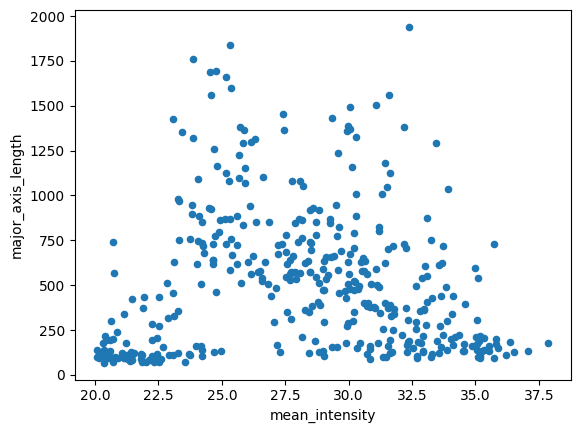

Next, we are going to split the data into a training subset of samples and a validation subset of samples. We can generate the machine learning model using the training samples, and then pick our best model using the validation samples.

In this way, we can keep the testing dataset clean (more on that in a second) and run experiments to pick the model we think will perform the best on previously unseen data.

We can use sklearn’s train_test_split function:

from sklearn.model_selection import train_test_split

# even though this is "test_size" it is coming from the training data in 'df'
df_train, df_val = train_test_split(df, test_size=0.1, train_size=0.9)

print("# training samples =", len(df_train))
print("# validation samples =", len(df_val))

# training samples = 359
# validation samples = 40

sklearn.clustering.KMeans

We can set up the KMeans model from sklearn using the following class methods and properties.

The KMeans class constructor (i.e., __init__) has several arguments, including:

n_clusters: number of clusters to generate
random_state: makes the “random” state repeatable by providing an integer value

The kmeans class instance has several properties, including

cluster_centers_ - the location (in feature space) of the cluster centers
labels_ - the labels for all of the input points (in the same order as the original samples)
interia_ - distances of each sample to their assigned cluster_centers_
n_features_in_ - size of the feature vector for each sample

Your Turn: Modify the clustering result by changing the two variables used for clustering and the KMeans parameters for the kmean instance. What are some things you notice when modifying each parameter? What is the impact (if any) of selecting to normalize (z-score) the data?

# @title Widget Code {"display-mode":"form"}
import numpy as np
import matplotlib.pyplot as plt

from sklearn.cluster import KMeans
from sklearn.preprocessing import StandardScaler
import ipywidgets as widgets
from IPython.display import display, clear_output
from matplotlib.colors import ListedColormap

OKABE_ITO = [
    "#000000", "#E69F00", "#56B4E9", "#009E73",
    "#F0E442", "#0072B2", "#D55E00", "#CC79A7"
]
cmap_okabe = ListedColormap(OKABE_ITO)

x_dd = widgets.Dropdown(options=numeric_cols, value=numeric_cols[0], description="X:")
y_dd = widgets.Dropdown(options=numeric_cols, value=numeric_cols[1], description="Y:")

k_slider = widgets.IntSlider(value=3, min=1, max=8, step=1, description="K:", continuous_update=False)
seed_box = widgets.IntText(value=0, description="seed:")
ninit_box = widgets.IntText(value=10, description="n_init:")

use_zscore = widgets.Checkbox(value=False, description="Z-score normalize (fit on df_train)")
show_val_names = widgets.Checkbox(value=True, description="Show label_name (df_val only)")
max_labels = widgets.IntSlider(value=5, min=0, max=40, step=5, description="Max labels:", continuous_update=False)

out = widgets.Output()

def _subset_indices(n_total, n_keep, seed):
    if n_keep >= n_total:
        return np.arange(n_total)
    rng = np.random.default_rng(seed)
    return rng.choice(n_total, size=n_keep, replace=False)

def plot_kmeans_train_val(xcol, ycol, K, seed, n_init, zscore, show_label_name_val, max_n_labels):
    if xcol == ycol:
        with out:
            clear_output(wait=True)
            print("Pick two different features for X and Y.")
        return

    Xtr_raw = df_train[[xcol, ycol]].to_numpy(dtype=np.float64)
    Xva_raw = df_val[[xcol, ycol]].to_numpy(dtype=np.float64)

    if zscore:
        scaler = StandardScaler()
        Xtr = scaler.fit_transform(Xtr_raw)
        Xva = scaler.transform(Xva_raw)
    else:
        Xtr, Xva = Xtr_raw, Xva_raw

    with out:
        clear_output(wait=True)

        km = KMeans(n_clusters=K, n_init=n_init, random_state=seed).fit(Xtr)

        ytr = km.labels_
        yva = km.predict(Xva)

        centers = km.cluster_centers_

        fig, axes = plt.subplots(1, 2, figsize=(13, 5), sharex=True, sharey=True)

        axes[0].scatter(
            Xtr[:, 0], Xtr[:, 1],
            c=ytr, cmap=cmap_okabe, vmin=-0.5, vmax=K-0.5,
            s=28, alpha=0.85, edgecolors="k", linewidths=0.25
        )
        axes[0].plot(centers[:, 0], centers[:, 1], "kx", markersize=10, label="cluster center")
        axes[0].set_title(f"TRAIN (fit) — K={K}")
        axes[0].legend(loc="best")

        axes[1].scatter(
            Xva[:, 0], Xva[:, 1],
            c=yva, cmap=cmap_okabe, vmin=-0.5, vmax=K-0.5,
            s=28, alpha=0.85, edgecolors="k", linewidths=0.25
        )
        axes[1].plot(centers[:, 0], centers[:, 1], "kx", markersize=10, label="cluster center")
        axes[1].set_title(f"VAL (predict) — K={K}")

        if show_label_name_val and ("label_name" in df_val.columns) and max_n_labels > 0:
            idx = _subset_indices(len(df_val), min(max_n_labels, len(df_val)), seed)
            for i in idx:
                axes[1].annotate(
                    str(df_val["label_name"].iloc[i]),
                    (Xva[i, 0], Xva[i, 1]),
                    xytext=(3, 3), textcoords="offset points",
                    fontsize=8, alpha=0.8
                )

        xlabel = f"{xcol}" + (" (z)" if zscore else "")
        ylabel = f"{ycol}" + (" (z)" if zscore else "")
        axes[0].set_xlabel(xlabel); axes[1].set_xlabel(xlabel)
        axes[0].set_ylabel(ylabel)

        plt.tight_layout()
        plt.show()
    return km


ui = widgets.VBox([
    widgets.HBox([x_dd, y_dd, k_slider, seed_box, ninit_box]),
    widgets.HBox([use_zscore, show_val_names, max_labels]),
])


display(ui, out)

widgets.interactive_output(
    plot_kmeans_train_val,
    {
        "xcol": x_dd,
        "ycol": y_dd,
        "K": k_slider,
        "seed": seed_box,
        "n_init": ninit_box,
        "zscore": use_zscore,
        "show_label_name_val": show_val_names,
        "max_n_labels": max_labels,
    },
)

Once you have selected your “perfect” clustering approach, we can test the data on an independent dataset. We do this to test the generalizability of the model.

These are some assumptions we can make when using separate training (and val) and testing datasets:

None of the data from the testing dataset were used to create the model
The testing and training datasets are representative of the population
If the testing and training datasets are independent*, performance on the testing dataset is an indicator of performance over the population

*Independence can be easily achieved using temporal splitting (“leave one year out”, etc.) Think about it: Why would this make the samples independent if they are from different years? Why would randomly grabbing samples from the same year potentially influence your performance?

We conveniently have labeled data, so we can directly examine the performance of your chosen KMeans model.

Think about it: Do the datapoints look like they could be from the same “population” as the training data?

import pandas as pd

df_test = pd.read_csv("storm_mode/sample_test_data.csv")

numeric_cols = df_test.select_dtypes(include="number").columns.tolist()
numeric_cols.remove('index')
numeric_cols.remove('label')
numeric_cols.remove('label1')

df_test.plot(kind='scatter', x='mean_intensity', y='major_axis_length')

<Axes: xlabel='mean_intensity', ylabel='major_axis_length'>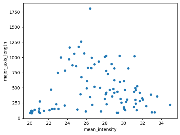

Let’s see how many unique labels exist in the dataset. If this differs from your model above, change it now!

df_test['label_name'].nunique()

5

We can ask the KMeans model to predict what cluster each sample belongs to. Just make sure to set your var1 and var2 below to match with your model above.

var1 = 'mean_intensity'
var2 = 'solidity'

num_cluster = 5
seed = 0
n_init = 10

df_train_x = df_train[[var1, var2]].to_numpy(dtype=np.float64)
df_test_x = df_test[[var1, var2]].to_numpy(dtype=np.float64)

kmeans = KMeans(n_clusters=num_cluster, n_init=n_init, random_state=seed).fit(df_train_x)

# the KMeans trained instance predicts the cluster
preds = kmeans.predict(df_test_x)

preds

array([1, 0, 3, 3, 1, 0, 1, 1, 1, 1, 1, 1, 0, 1, 0, 3, 0, 1, 1, 1, 1, 3,
       1, 1, 0, 0, 1, 1, 0, 1, 0, 1, 1, 4, 0, 4, 1, 3, 4, 1, 0, 0, 0, 1,
       0, 4, 0, 1, 1, 0, 0, 0, 0, 0, 0, 0, 0, 4, 0, 1, 4, 4, 0, 4, 0, 4,
       4, 4, 4, 4, 4, 4, 0, 0, 2, 0, 4, 4, 4, 0, 2, 2, 2, 2, 2, 2, 2, 2,
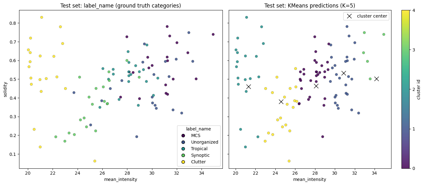
       4, 2, 2, 4, 2, 2, 2, 2, 2, 2, 2, 2], dtype=int32)

Results:

import numpy as np
import matplotlib.pyplot as plt

centers = kmeans.cluster_centers_

fig, axes = plt.subplots(1, 2, figsize=(14, 6), sharex=True, sharey=True)

name_codes, name_levels = pd.factorize(df_test["label_name"])

sc0 = axes[0].scatter(
    df_test[var1], df_test[var2],
    c=name_codes,
    s=35, alpha=0.85,
    edgecolors="k", linewidths=0.25
)
axes[0].set_title("Test set: label_name (ground truth categories)")
axes[0].set_xlabel(var1)
axes[0].set_ylabel(var2)

handles0 = []
for code, name in enumerate(name_levels):
    handles0.append(plt.Line2D([0], [0], marker="o", linestyle="",
                               markerfacecolor=sc0.cmap(sc0.norm(code)),
                               markeredgecolor="k", markersize=7, label=str(name)))
if len(handles0) <= 15:
    axes[0].legend(handles=handles0, title="label_name", loc="best")

sc1 = axes[1].scatter(
    df_test[var1], df_test[var2],
    c=preds,
    s=35, alpha=0.85,
    edgecolors="k", linewidths=0.25
)
axes[1].plot(centers[:, 0], centers[:, 1], "kx", markersize=10, label="cluster center")
axes[1].set_title(f"Test set: KMeans predictions (K={num_cluster})")
axes[1].set_xlabel(var1)
axes[1].legend(loc="best")

cbar = fig.colorbar(sc1, ax=axes[1], ticks=np.arange(num_cluster))
cbar.set_label("cluster id")

plt.tight_layout()
plt.show()

Lab 6 will further explore performance metrics using these datasets

Chapter 8.2.2 - Self-organizing Map¶

The self-organizing map (SOM) is a type of unsupervised machine learning approach that transforms high-dimensional data (e.g., 2D images) into a low-dimensional representation (e.g., a node). For example, you could take hundreds or thousands of 500 hPa height fields and organize them into nodes where the data within each node are most similar to one another, but they are also more similar to the nearby nodes compare to nodes farther away.

Similar to KMeans clustering, the SOM produces a given number of nodes (clusters). The main differences between the SOM and KMeans are:

The SOM requires the user to define the size of a 2D grid on which the SOM will organize clusters (i.e., y-count and x-count). KMeans only requires a single number.
The nodes (clusters) in the SOM are organized in a way that the nearest nodes are more similar than nodes farther away in the grid.

The SOM learning approach is initialized with random M x N “weights” that are the same dimensions as your input data. For example, a 16-feature vector on a 5x5 SOM grid would produce 25 weight vectors associated with each node. The weights will test how “similar” a sample is to some “prototype vector” that is slowly tuned based on samples being passed into the model training step. We will talk more about neural networks later in the course, and will focus on applying SOM in Geoscience applications.

SVRIMG

We will apply SOMs using the SVRIMG dataset. This dataset is comprised of thousands of radar images that are centered on severe weather reports. The goal of this part of the chapter is to see if we can cluster the radar images into groups that are similar to the manually-labeled storm shapes defined by SVRIMG.

The following code will download 1 year of data (2011).

%%bash
pip install cmweather  > /dev/null
pip install minisom > /dev/null
mkdir svrimg
cd svrimg
wget -nc -q https://nimbus.niu.edu/svrimg/data/tars/tor/2011_svrimg_raw.tar.gz  > /dev/null
wget -nc -q https://nimbus.niu.edu/svrimg/data/tars/tor/2008_svrimg_raw.tar.gz  > /dev/null
tar -xzf 2011_svrimg_raw.tar.gz  > /dev/null
tar -xzf 2008_svrimg_raw.tar.gz  > /dev/null

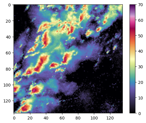
We can visualize these data and see they are radar image snapshots:

from imageio import imread
import matplotlib.pyplot as plt
import cmweather
import numpy as np

img = imread("/content/svrimg/2011/04/201104272213z000293961.png", pilmode='P')

plt.imshow(np.flipud(img), cmap='ChaseSpectral', vmin=0, vmax=70)
plt.colorbar()

/tmp/ipython-input-652088369.py:6: DeprecationWarning: Starting with ImageIO v3 the behavior of this function will switch to that of iio.v3.imread. To keep the current behavior (and make this warning disappear) use `import imageio.v2 as imageio` or call `imageio.v2.imread` directly.
  img = imread("/content/svrimg/2011/04/201104272213z000293961.png", pilmode='P')

We first need to preprocess the images to read them in and flatten them. SOM training requires a 1D feature vector and these images are 2D. We find that we have 1,690 images, and each feature vector is 18,496 features long.

import glob
import numpy as np

imgs = []

# the * says give me everything in that folder
for fname in glob.glob("/content/svrimg/2011/*/*.png"):
    img = imread(fname, pilmode='P')
    imgs.append(np.flipud(img).flatten())

X = np.asarray(imgs, dtype=np.float32)

print("The number of svrimg images is: ", X.shape)

/tmp/ipython-input-2132654484.py:8: DeprecationWarning: Starting with ImageIO v3 the behavior of this function will switch to that of iio.v3.imread. To keep the current behavior (and make this warning disappear) use `import imageio.v2 as imageio` or call `imageio.v2.imread` directly.
  img = imread(fname, pilmode='P')

The number of svrimg images is:  (1690, 18496)

We will use the minisom package to cluster the radar images. I have also downloaded a ‘helper’ python script to make the training process easier. We will normalize the dBZ values using the z-score calculation from scikit-learn processing to improve model performance.

from sklearn.preprocessing import StandardScaler

scaler = StandardScaler()
Xz = scaler.fit_transform(X)

Next, we set the SOM parameters. You can feel free to modify these to see how they change the result.

m, n = 4, 4
sigma = 2.0
learning_rate = 0.1
seed = 0

Finally, we train the MiniSom model using our standardized data.


from minisom import MiniSom

som = MiniSom(
    x=m, y=n,
    input_len=len(X[0]),
    sigma=sigma,
    learning_rate=learning_rate,
    neighborhood_function="gaussian",
    random_seed=seed
)

num_iterations = 10000

som.random_weights_init(Xz)
som.train_random(Xz, num_iterations, verbose=True)

bmus = np.array([som.winner(x) for x in Xz])
bmu_flat = bmus[:, 0] * n + bmus[:, 1]

print("BMU coords for first 10 samples:", bmus[:10])
print("Unique BMUs used:", len(np.unique(bmu_flat)))

 [ 10000 / 10000 ] 100% - 0:00:00 left 
 quantization error: 109.62333698834476
BMU coords for first 10 samples: [[3 3]
 [3 3]
 [1 2]
 [3 3]
 [2 1]
 [2 2]
 [1 2]
 [3 3]
 [1 2]
 [1 2]]
Unique BMUs used: 16

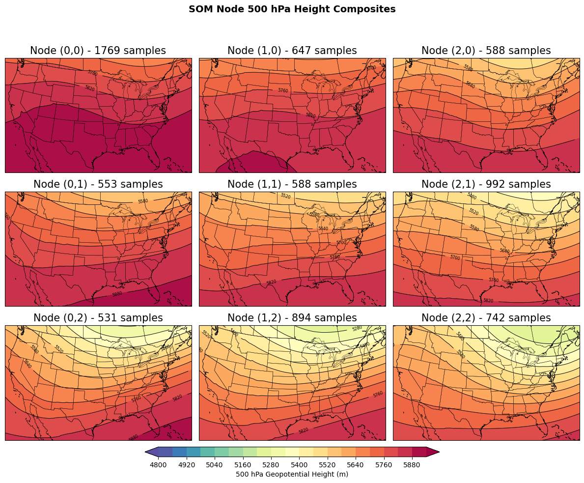
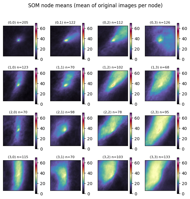
Once trained, we can step through each node and find the ‘winner’ (node #) assigned to each sample. We then find the mean of the samples and plot them on the graph below. This is a simple way to quickly examine the shape and intensity of samples assigned to each node.

Your turn: What do you notice about each node?

import numpy as np
import matplotlib.pyplot as plt

X = np.asarray(imgs, dtype=np.float32)
Xz = scaler.transform(X)

N, P = X.shape

side = int(np.sqrt(P))
img_shape = (side, side)

bmus = np.array([som.winner(x) for x in Xz], dtype=int)

sums = np.zeros((m, n, P), dtype=np.float64)
counts = np.zeros((m, n), dtype=np.int64)

for i, (r, c) in enumerate(bmus):
    sums[r, c] += X[i]
    counts[r, c] += 1

means = np.zeros((m, n, P), dtype=np.float32)
nonempty = counts > 0
means[nonempty] = (sums[nonempty] / counts[nonempty, None]).astype(np.float32)

fig, axes = plt.subplots(m, n, figsize=(1.6 * n, 1.6 * m), squeeze=False)

valid = means[nonempty].reshape(-1)

for r in range(m):
    for c in range(n):
        ax = axes[r, c]
        if counts[r, c] > 0:
            mmp = ax.imshow(means[r, c].reshape(img_shape), vmin=0, vmax=70, cmap='ChaseSpectral')
            ax.set_title(f"({r},{c}) n={counts[r,c]}", fontsize=8)
        else:
            ax.set_facecolor("0.9")
            ax.set_title(f"({r},{c}) n=0", fontsize=8)
        ax.set_xticks([])
        ax.set_yticks([])
        plt.colorbar(mmp, ax=ax)

plt.suptitle("SOM node means (mean of original images per node)", y=1.02)
plt.tight_layout()

Your turn: Try to read in data from another year and assign nodes to those examples:

import glob
import numpy as np

imgs08 = []

# the * says give me everything in that folder
for fname in glob.glob("/content/svrimg/2008/*/*.png"):
    img = imread(fname, pilmode='P')
    imgs08.append(np.flipud(img).flatten())

X08 = np.asarray(imgs08, dtype=np.float32)

print("The number of svrimg images is: ", X08.shape)

/tmp/ipython-input-2777955933.py:8: DeprecationWarning: Starting with ImageIO v3 the behavior of this function will switch to that of iio.v3.imread. To keep the current behavior (and make this warning disappear) use `import imageio.v2 as imageio` or call `imageio.v2.imread` directly.
  img = imread(fname, pilmode='P')

The number of svrimg images is:  (1687, 18496)