%%bash

pip install rasterio
pip install pillow
pip install cmweather
wget -nc -q https://nimbus.niu.edu/courses/EAE483/BREF_090508_1300.png
wget -nc -q https://nimbus.niu.edu/courses/EAE483/000000274089.tif
Requirement already satisfied: rasterio in /usr/local/lib/python3.12/dist-packages (1.5.0)
Requirement already satisfied: affine in /usr/local/lib/python3.12/dist-packages (from rasterio) (2.4.0)
Requirement already satisfied: attrs in /usr/local/lib/python3.12/dist-packages (from rasterio) (25.4.0)
Requirement already satisfied: certifi in /usr/local/lib/python3.12/dist-packages (from rasterio) (2026.2.25)
Requirement already satisfied: click!=8.2.*,>=4.0 in /usr/local/lib/python3.12/dist-packages (from rasterio) (8.3.1)
Requirement already satisfied: cligj>=0.5 in /usr/local/lib/python3.12/dist-packages (from rasterio) (0.7.2)
Requirement already satisfied: numpy>=2 in /usr/local/lib/python3.12/dist-packages (from rasterio) (2.0.2)
Requirement already satisfied: pyparsing in /usr/local/lib/python3.12/dist-packages (from rasterio) (3.3.2)
Requirement already satisfied: pillow in /usr/local/lib/python3.12/dist-packages (11.3.0)
Collecting cmweather
Downloading cmweather-0.3.2-py3-none-any.whl.metadata (2.9 kB)
Requirement already satisfied: numpy in /usr/local/lib/python3.12/dist-packages (from cmweather) (2.0.2)
Requirement already satisfied: matplotlib in /usr/local/lib/python3.12/dist-packages (from cmweather) (3.10.0)
Requirement already satisfied: contourpy>=1.0.1 in /usr/local/lib/python3.12/dist-packages (from matplotlib->cmweather) (1.3.3)
Requirement already satisfied: cycler>=0.10 in /usr/local/lib/python3.12/dist-packages (from matplotlib->cmweather) (0.12.1)
Requirement already satisfied: fonttools>=4.22.0 in /usr/local/lib/python3.12/dist-packages (from matplotlib->cmweather) (4.62.1)
Requirement already satisfied: kiwisolver>=1.3.1 in /usr/local/lib/python3.12/dist-packages (from matplotlib->cmweather) (1.5.0)
Requirement already satisfied: packaging>=20.0 in /usr/local/lib/python3.12/dist-packages (from matplotlib->cmweather) (26.0)
Requirement already satisfied: pillow>=8 in /usr/local/lib/python3.12/dist-packages (from matplotlib->cmweather) (11.3.0)
Requirement already satisfied: pyparsing>=2.3.1 in /usr/local/lib/python3.12/dist-packages (from matplotlib->cmweather) (3.3.2)
Requirement already satisfied: python-dateutil>=2.7 in /usr/local/lib/python3.12/dist-packages (from matplotlib->cmweather) (2.9.0.post0)
Requirement already satisfied: six>=1.5 in /usr/local/lib/python3.12/dist-packages (from python-dateutil>=2.7->matplotlib->cmweather) (1.17.0)
Downloading cmweather-0.3.2-py3-none-any.whl (47 kB)
━━━━━━━━━━━━━━━━━━━━━━━━━━━━━━━━━━━━━━━━ 47.3/47.3 kB 1.9 MB/s eta 0:00:00
Installing collected packages: cmweather
Successfully installed cmweather-0.3.2
Chapter 9.1 - Digital Image Processing
Digital image processing describes a set of algorithms that can be used to manipulate digital images. Many of these algorithms are foundational for deep learning and other modern machine learning approaches. In this chapter, we will introduce how images are represented in computer systems, visualization and interpretation of digital images, common algorithms used to modify these images, and machine learning models that work with images.
Chapter 9.1.1 - What is a digital image?
In a previous chapter, we introduced the raster data model. We learned that, in Python, rasters are represented as numeric arrays of two or more dimensions. Each number in the raster represents the value within a grid cell. Each grid cell represents some region from which a measurement was taken. For example, when taking a picture with a camera, each pixel is representing the intensity detected by the camera’s sensor in certain spectral bands.
Humans perceive colors using specialized cells on our retinas called cones. Each cone is more sensitive to relative visible frequencies--namely, the S cone (400-500 nm), M cone (450-630 nm), and L cone (500-700 nm). While these are commonly connected to the wavelength at which they are most sensitive--blue (420 nm), green (534 nm), and red (564 nm), respectively--the actual sensitivity is better represented by a spectrum centered on those colors. For example, M and L cones are sensitive to green and red.
Chapter 9.1.2 - RGB Color Model
That said, the so-called “RGB” color model is based on a simplification of the human visual system. Information from sensors (e.g., cameras, satellite platforms, etc.) are processed based on the intensity of light at the red, green, and blue wavelengths. In the raster data model, this requires the array to be three dimensional--two dimensions for space (e.g., x and y), and one dimension for the individual intensities of red, green, or blue light captured by the sensor. The third dimension of the RGB color model is often called a “channel”. If a pixel value has a non-zero intensity for the red channel and a zero intensity for the green and blue channels, the pixel will be assigned the color red. A healthy combination of green and red channel intensities, with no blue intensity, will produce a yellow, etc.
Hexadecimal and Decimal Encoding
In an 8-bit RGB image, each pixel stores three integers: one for red, one for green, and one for blue. Each channel ranges from 0 to 255, so one pixel can be written as (R, G, B), such as (0, 128, 255). The same color can also be written in hexadecimal form as #RRGGBB, where each pair of hex digits encodes one channel. For example, #FFFFFF corresponds to (255, 255, 255) and #000000 corresponds to (0, 0, 0).
You may also see colors encoded as a hexadecimal value. A hexadecimal value (or “hex code”; e.g., #FF0000) is often used to encode specific colors using 8 bits (1 byte) to store each color intensity--specifically:
| Channel | Digits | Size | HEX example for ‘black’ | Equivalent Raw Binary for ‘black’ (disk storage) |
|---|---|---|---|---|
| Red | 1-2 | 8 bits | 00 | 00000000 |
| Green | 3-4 | 8 bits | 00 | 00000000 |
| Blue | 5-6 | 8 bits | 00 | 00000000 |
In other words, 1 pixel of raw RGB information stored on a disk (uncompressed) will take up 3 bytes (24 bits) of space. Black, for example, can be represented through a hexadecimal as 000000, and in binary as:
00000000 00000000 00000000
Each two-digit sequence can encode 256 different intensities for each color, and the 3 sequences together encode more than 16 million unique colors. A nice website for exploring colormaps and generating hex codes is ColorBrewer: https://
The maximum hex value (FF) for any color is equivalent to an integer of 255. So, using the hex code of #FFFFFF for a color is equivalent to an RGB array of (255, 255, 255).
Hexadecimal values use a base-16 numbering system. We typically use a base-10 system, where all possible numbers are just combinations of the digits 0-9. Conversions from base-16 (hexadecimal) to base-10 (decimal) for one digit is as follows:
| Hexadecimal | Decimal |
|---|---|
| 0 | 0 |
| 1 | 1 |
| 2 | 2 |
| 3 | 3 |
| 4 | 4 |
| 5 | 5 |
| 6 | 6 |
| 7 | 7 |
| 8 | 8 |
| 9 | 9 |
| A | 10 |
| B | 11 |
| C | 12 |
| D | 13 |
| E | 14 |
| F | 15 |
To get the number 16, we just repeat the cycle by adding another digit. We set the first digit to 1, and the second digit to 0. This results in an unintuitive solution!
10
This unintuitively is equivalent to 16 in base-10.
For two digits, the hex-to-base-10 conversion, after converting each digit to a value between 0 and 15, is as follows:
base10 = (first_digit * 16**1) + (second_digit * 16**0)The exponents increment for every additional digit. For example, if you have three digits 1F1:
base16_to_10 = (1 * 16**2) + (15 * 16**1) + (1 * 16**0)This is equivalent to 497 in decimal.
This seems odd until you realize that going from 9 to 10 is just repeating the base-10 cycle when you run out of digits:
256 in base-10 can be described using the same equation above:
base10_expansion = (2 * 10**2) + (5 * 10**1) + (6 * 10**0)This might make binary or base-2 make more sense to you. This is how computers store data types like integers. If we assume that each digit is going to be multiplied by 2$^{n}, where n is the number of digits, that makes storing values very convenient in a system that was designed to send “on” and “off” signals to transfer and process data.
So, 10 in binary is what in decimal? 2!
base2_to_10 = (1 * 2**1) + (0 * 2**0)So, the digits 10 can be a value of:
10inbase-1016inbase-162inbase-2
Other common base types include:
less intuitive, but maps the numbers 0 - 63 to various letters and symbols. E.g.,
0isA,62is ‘+’, etc.
When setting permissions with commands like
chmod, you specify three digits in the order owner, group, and others. For each digit, permissions are calculated as the sum of the values read (4), write (2), and execute (1). The owner is the user who owns the file or directory, the group refers to the file’s assigned group, and others includes everyone who is neither the owner nor a member of that assigned group.755means: the owner gets read, write, and execute (4 + 2 + 1 = 7), the group gets read and execute (4 + 1 = 5), and others get read and execute (4 + 1 = 5).
Image Compression
Before, we discussed that we can store a pixel value representing a color on disk in 24-bit binary form that takes up 3 bytes of data:
00000000 00000000 00000000
If we instead store the image in grayscale, we could reduce the size of each pixel to 8-bits (1 byte):
00000000
Grayscale images are commonly used in geoscience applications. For example, the radar images we examined in previous chapters were grayscale, 8-bit images that only used a fraction of the 8-bit int space (e.g., 0 - ~80 dBZ). If we used color quantization, we could potentially encode ranges of 5 dBZ into 16 values (0 - 16) and pack them into a 4 bit image. However, Python (specifically, numpy) only provides an 8-bit int type.
Try it yourself: We can examine the values of a grayscale radar image below. What are the differences between the grayscale image and the RGB image?
import matplotlib.pyplot as plt

import cmweather
import numpy as np
from PIL import Image

plt.rcParams['figure.figsize'] = 10, 10

img = Image.open("BREF_090508_1300.png")
img = np.array(img)

print(img.shape)

plt.imshow(np.array(img) * 5, cmap='ChaseSpectral')
plt.title("Radar Reflectivity (May 8th 2009 13:00:00 UTC)")
cbar = plt.colorbar(shrink=0.25)
cbar.set_label("dBZ")

print(img)
(1837, 3661)
[[0 0 0 ... 0 0 0]
[0 0 0 ... 0 0 0]
[0 0 0 ... 0 0 0]
...
[0 0 0 ... 0 0 0]
[0 0 0 ... 0 0 0]
[0 0 0 ... 0 0 0]]
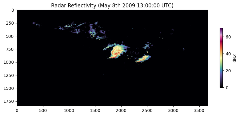
Interestingly, the grayscale radar image is smaller in size on disk (67.29 KB) compared to the RGB geotiff (198 KB), despite having the dimensions of (1837, 3661) vs. (128, 128, 3).
from pathlib import Path

path = Path("BREF_090508_1300.png")
size_bytes = path.stat().st_size

print(f"Gray Bytes: {size_bytes}")
print(f"Gray KB: {size_bytes / 1024:.2f}")
print(f"Gray MB: {size_bytes / (1024**2):.4f}")

from pathlib import Path

path = Path("000000274089.tif")
size_bytes = path.stat().st_size

print(f"RGB Bytes: {size_bytes}")
print(f"RGB KB: {size_bytes / 1024:.2f}")
print(f"RGB MB: {size_bytes / (1024**2):.4f}")
Gray Bytes: 68900
Gray KB: 67.29
Gray MB: 0.0657
RGB Bytes: 203399
RGB KB: 198.63
RGB MB: 0.1940
While the 8-bit vs. 24-bit tells part of the story, the other part is in how the png (Portable Network Graphics) compression works.
There are two types of compression algorithms:
lossless: the original pixel values can be recovered after compressionlossy: the original pixel values are only approximately recovered after compression (e.g., JPEG)
The distinction is very important. JPEG might work for storing family photos, but might be too destructive for geoscience data. For example, the JPEG compression is a multi-step process that tries to eliminate unneeded data in an image. While the compression results are impressive, legitimate data can be lost forever.
In contrast, PNG works by identifying runs in images and transforming rows of values into sequences of:
(how many times does the value repeat, repeated value)
For example, consider one row of a grayscale image:
0, 0, 0, 0, 0, 0, 255, 255, 255, 255, 255, 0, 0, 0
could be stored as a representation that resembles this:
6, 0, 5, 255, 3, 0
The PNG decoder would know that all odd values are the repeat count, and the even numbers are the repeated value.
Try it yourself: Try to write a png encoder that can convert one 8-bit line into a compressed representation.
raw_values = np.array([0, 0, 0, 0, 0, 0, 255, 255, 255, 255, 255, 0, 0, 0])Try it yourself: Using what you know about hexadecimal and decimal values, modify the RGB array values (i.e., decimal) below to get the following hexadecimal values. What colors do they represent?
#FFFFFF#FF0000#00FF00#0000FF#000000
Try it yourself: Based on the color blending figure above, approximately create the following colors. What hexadecimal and RGB decimal codes most closely match to those colors?
OrangeYellowPurpleGrey
import numpy as np
import matplotlib.pyplot as plt
import ipywidgets as widgets
from IPython.display import display

def show_pixel(r=128, g=128, b=128):
    pixel = np.array([[[r, g, b]]], dtype=np.uint8)
    hex_color = f"#{r:02X}{g:02X}{b:02X}"

    fig, ax = plt.subplots(figsize=(4, 4))
    ax.imshow(pixel, interpolation='nearest')
    ax.set_title(f"RGB = ({r}, {g}, {b})\n{hex_color}", fontsize=14)
    ax.set_xticks([])
    ax.set_yticks([])
    plt.show()

r_slider = widgets.IntSlider(value=128, min=0, max=255, step=1, description='R')
g_slider = widgets.IntSlider(value=128, min=0, max=255, step=1, description='G')
b_slider = widgets.IntSlider(value=128, min=0, max=255, step=1, description='B')

widgets.interact(show_pixel, r=r_slider, g=g_slider, b=b_slider);Single-pixel HSV Image
The HSV (Hue, Saturation, Value) color model is similar, but instead encodes images using:
Hue — the basic color type, such as red, orange, yellow, green, blue, or violet.
Saturation — how vivid or pure the color is, ranging from gray and dull to rich and intense.
Value — the brightness of the color, ranging from dark to bright.
You can modify the HSV values below to get a particular color. Notice that the colorsys package converts HSV to RGB. Much like the decimal system, the RGB system serves as the universal color system for matplotlib.
import numpy as np
import matplotlib.pyplot as plt
import ipywidgets as widgets
import colorsys

def show_hsv_patch(h=180, s=0.5, v=0.5):
    r, g, b = colorsys.hsv_to_rgb(h / 360.0, s, v)
    patch = np.ones((50, 50, 3), dtype=float)
    patch[..., 0] = r
    patch[..., 1] = g
    patch[..., 2] = b

    r255 = int(round(r * 255))
    g255 = int(round(g * 255))
    b255 = int(round(b * 255))

    hex_color = f"#{r255:02X}{g255:02X}{b255:02X}"

    fig, ax = plt.subplots(figsize=(6, 6))
    ax.imshow(patch)
    ax.set_title(f"HSV=({h:.0f}, {s:.2f}, {v:.2f})\nRGB=({r255}, {g255}, {b255})\n{hex_color}")
    ax.set_xticks([])
    ax.set_yticks([])
    plt.show()

widgets.interact(
    show_hsv_patch,
    h=widgets.IntSlider(value=180, min=0, max=360, step=1, description='H'),
    s=widgets.FloatSlider(value=0.5, min=0, max=1, step=0.01, description='S'),
    v=widgets.FloatSlider(value=0.5, min=0, max=1, step=0.01, description='V')
);Try it yourself
Modify the following 4 pixel array (2x2) named color_arr to display the colors red, green, blue, and black
color_arr = [[(128, 128, 128), (128, 128, 128)],
             [(128, 128, 128), (128, 128, 128)]]


pixels = np.array(color_arr)

fig, ax = plt.subplots(figsize=(6, 6))
ax.imshow(pixels, interpolation='nearest')
ax.set_title("2x2 color array", fontsize=14)
ax.set_xticks([0.5, 1.5])
ax.set_yticks([0.5, 1.5])
ax.set_yticklabels([])
ax.set_xticklabels([])
plt.grid()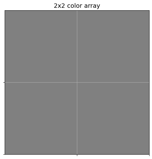
Real world RGB Example
The United States Geological Survey (USGS) has a repository of NAIP (National Agriculture Imagery Program) imagery. These images are RGB composites collected by sensors on aircraft, and offer a resoluton of 0.6 m (or better) per grid. This dataset is primarily to monitor crops during the growing season. However, there are many other applications of these data, including building and event detection.
We can read in these data using rasterio. When you display the data contained within the array arr, you can see it is just a 3D array of values ranging from 0 - 255. The first dimension is the channel (RGB), the 2nd dimension is y (i.e., northing), and the 3rd dimension is x (i.e., easting).
import rasterio

tif_path = "000000274089.tif"

with rasterio.open(tif_path) as src:
    arr = src.read()
    profile = src.profile

print("Array shape:", arr.shape)
print("Data type:", arr.dtype)
print("Profile:")
print(profile)

print(arr)
Array shape: (3, 256, 256)
Data type: uint8
Profile:
{'driver': 'GTiff', 'dtype': 'uint8', 'nodata': None, 'width': 256, 'height': 256, 'count': 3, 'crs': CRS.from_wkt('PROJCS["NAD83 / UTM zone 16N",GEOGCS["NAD83",DATUM["North_American_Datum_1983",SPHEROID["GRS 1980",6378137,298.257222101004,AUTHORITY["EPSG","7019"]],AUTHORITY["EPSG","6269"]],PRIMEM["Greenwich",0],UNIT["degree",0.0174532925199433,AUTHORITY["EPSG","9122"]],AUTHORITY["EPSG","4269"]],PROJECTION["Transverse_Mercator"],PARAMETER["latitude_of_origin",0],PARAMETER["central_meridian",-87],PARAMETER["scale_factor",0.9996],PARAMETER["false_easting",500000],PARAMETER["false_northing",0],UNIT["metre",1,AUTHORITY["EPSG","9001"]],AXIS["Easting",EAST],AXIS["Northing",NORTH],AUTHORITY["EPSG","26916"]]'), 'transform': Affine(0.5999999999999996, 0.0, 633510.0,
0.0, -0.6000000000999995, 3665995.199991812), 'blockxsize': 128, 'blockysize': 128, 'tiled': True, 'compress': 'lzw', 'interleave': 'pixel'}
[[[170 138 105 ... 157 159 161]
[168 141 114 ... 163 164 165]
[166 145 124 ... 168 168 168]
...
[102 102 101 ... 99 104 109]
[ 94 103 112 ... 105 106 106]
[ 86 98 109 ... 110 107 104]]
[[182 151 120 ... 164 166 168]
[178 153 128 ... 170 171 172]
[175 156 136 ... 176 176 175]
...
[122 120 118 ... 107 112 117]
[114 121 128 ... 114 114 114]
[105 115 125 ... 120 115 110]]
[[158 130 102 ... 108 114 120]
[152 129 106 ... 111 116 122]
[146 128 109 ... 114 119 124]
...
[120 117 114 ... 90 94 97]
[110 116 123 ... 96 95 94]
[ 99 108 118 ... 102 97 92]]]
We can plot these data using matplotlib, but we first need to transpose the data into a different orientation of dimensions. matplotlib requires RGB data to be organized with channels as the last dimension. It can be difficult to figure out how to shuffle the data dimensions around. Luckily, numpy has a built-in transpose function:
rgb = np.transpose(arr, (1, 2, 0)Where the first argument is the original array, the 2nd argument is the new order of dimensions. In other words, (1, 2, 0) when passed into this method will do the following conversion that sets it up nicely for matplotlib.
| Original | transpose |
|---|---|
| 0 | 1 |
| 1 | 2 |
| 2 | 0 |
Try it yourself: Use the widgets below to modify the R, G, and/or B channels with a fractional adjustment, where 2 is 200% and 0 is 0%. Are there any details about the image that are more / less obvious if a channel is dampened (scale < 1) or amplified (scale > 1)?
rgb = np.transpose(arr[:3], (1, 2, 0))

def adjust_rgb(r_scale=1.0, g_scale=1.0, b_scale=1.0):
    out = rgb.astype(np.float32).copy()

    out[:,:,0] *= r_scale
    out[:,:, 1] *= g_scale
    out[:,:, 2] *= b_scale

    out = np.clip(out, 0, 255).astype(np.uint8)

    plt.figure(figsize=(5, 5))
    plt.imshow(out)
    plt.title(f"R × {r_scale:.2f}, G × {g_scale:.2f}, B × {b_scale:.2f}")
    plt.axis("off")
    plt.show()

widgets.interact(
    adjust_rgb,
    r_scale=widgets.FloatSlider(value=1.0, min=0.0, max=2.0, step=0.01, description='R'),
    g_scale=widgets.FloatSlider(value=1.0, min=0.0, max=2.0, step=0.01, description='G'),
    b_scale=widgets.FloatSlider(value=1.0, min=0.0, max=2.0, step=0.01, description='B'),
);