%%bash
pip install cartopy > /dev/null
pip install geopandas > /dev/null

Chapter 7.3 - Vector Data Analysis¶

As we discussed in previous sections in this chapter, geographic data can be organized into raster and vector data. This section will be dedicated to an introduction to vector data analysis. A full treatment of this topic would require taking a Geographic Information Systems (GIS) course.

As you may recall, vector data include points, polygons, and other shapes that represent a position, boundary/edge, or area. Common vector data analyses include manipulation of the geographic data itself (e.g., buffering, clipping, merging, etc.) and spatial selections (e.g., spatial joins, etc.). Your job as a Geoscientist is to figure out how to translate these basic GIS techniques into workflows that manipulate the data in a way that is physically meaninful and logical.

Chapter 7.3.1 - Buffering¶

We introduced the idea of buffering in a previous section in this chapter. This process takes the original geometry and increases its extent by a distance defined by the user and controlled by the coordinate system. This process is rarely used on its own. Often, you define a buffer to select a subset of other geographic data. For example, imagine a situation like the Chernobyl Nuclear Disaster. The reactor failures occurred in a relatively small area (e.g., the lat/lon position of the power plant), but clearly had “influence” on a much larger area when considering potential radiation exposure.

You might also try to answer a question about risk for a location (e.g., your house, a school, etc.) by identifying hazards that have occurred within a certain distance of that location.

Consider the following situation: You are an administrator for NIU. You need to decide on the relative tornado risk for NIU. You decide that you want to know how many tornadoes occurred within 25 miles (~40 km) of the university.

Here are the raw geographic data:

%%bash
wget -q -nc https://www.spc.noaa.gov/wcm/data/1950-2024_actual_tornadoes.csv > /dev/null

Tornado data from the Storm Prediction Center:

import pandas as pd

tornadoes = pd.read_csv("1950-2024_actual_tornadoes.csv")

tornadoes

NIU location:

from shapely.geometry import Point

niu = Point(-88.7739, 41.9342)

What are some of the considerations associated with connecting these two data sources?

Conversion to shapely/geopandas to use the geographic methods
Definition of the projection
Conversion to a projected coordinate system (if needed)
Translating the Geoscience need to a GIS workflow
Validating the results through visualization
Performing the statistical analysis on the resulting data.

Converting the “raw” data to geopandas

The single point is relatively straightforward. You simply need to define some attribute data using a dictionary and then set the geometry argument to the point in the GeoDataFrame constructor. We place NIU and niu in a list because the GeoDataFrame is expecting an iterable since you usually will have multiple rows of attributes and geometry.

import geopandas as gpd

niu = gpd.GeoDataFrame({"location": ['NIU']}, geometry=[niu])

niu

We can do the same thing with the tornado data, except we have a lot of premade columns and rows, so the manual insertion we did in the previous step is not needed.

The complex part about this step is getting the lat/lon information into a format that Geopandas can use. As was the case in the previous step, this requires us to make a list of Point.

If you examine the dataset, you will note that the columns include a slon and slat. These represent the starting points of the tornadoes.

tornadoes[['slon', 'slat']]

We need to loop through these lat/lon pairs, transform each pair into a Point, and save that point in a list. Luckily, Geopandas has a method for this called points_from_xy.

This method expects a list of x and y points, where the x and y pairs are identified by the order they exist within the list. In other words, the slon at index 5 is paired with the slat at index 5.

We can get separate lists like this:

lons = tornadoes['slon']
lats = tornadoes['slat']

print("these are the lons ->", lons)
print("\nthese are the lats ->", lats)

these are the lons -> 0       -102.5200
1        -78.6000
2        -87.2000
3        -84.5000
4        -89.1300
           ...   
71808    -86.9567
71809   -108.2136
71810    -79.0102
71811    -75.8837
71812    -78.3987
Name: slon, Length: 71813, dtype: float64

these are the lats -> 0        36.7300
1        34.1700
2        37.3700
3        38.2000
4        32.4200
          ...   
71808    41.7019
71809    43.6457
71810    43.0333
71811    43.7565
71812    43.0241
Name: slat, Length: 71813, dtype: float64

and we can use points_from_xy like this. The result is a GeometryArray of Point, which can be used directly during the creation of a GeoDataFrame.

pts = gpd.points_from_xy(lons, lats)

pts

<GeometryArray>
[  <POINT (-102.52 36.73)>,     <POINT (-78.6 34.17)>,
     <POINT (-87.2 37.37)>,      <POINT (-84.5 38.2)>,
    <POINT (-89.13 32.42)>,     <POINT (-76.12 40.2)>,
    <POINT (-90.05 38.97)>,    <POINT (-89.67 38.75)>,
    <POINT (-91.83 36.12)>,    <POINT (-89.78 38.17)>,
 ...
  <POINT (-78.488 36.319)>,    <POINT (-81.43 30.67)>,
 <POINT (-109.875 42.638)>,  <POINT (-98.101 35.841)>,
  <POINT (-78.176 42.135)>,  <POINT (-86.957 41.702)>,
 <POINT (-108.214 43.646)>,   <POINT (-79.01 43.033)>,
  <POINT (-75.884 43.756)>,  <POINT (-78.399 43.024)>]
Length: 71813, dtype: geometry

We can even add projection information during this step by assigning a lat/lon projection to the points:

pts = gpd.points_from_xy(lons, lats, crs='EPSG:4269')

pts.crs

<Geographic 2D CRS: EPSG:4269>
Name: NAD83
Axis Info [ellipsoidal]:
- Lat[north]: Geodetic latitude (degree)
- Lon[east]: Geodetic longitude (degree)
Area of Use:
- name: North America - onshore and offshore: Canada - Alberta; British Columbia; Manitoba; New Brunswick; Newfoundland and Labrador; Northwest Territories; Nova Scotia; Nunavut; Ontario; Prince Edward Island; Quebec; Saskatchewan; Yukon. Puerto Rico. United States (USA) - Alabama; Alaska; Arizona; Arkansas; California; Colorado; Connecticut; Delaware; Florida; Georgia; Hawaii; Idaho; Illinois; Indiana; Iowa; Kansas; Kentucky; Louisiana; Maine; Maryland; Massachusetts; Michigan; Minnesota; Mississippi; Missouri; Montana; Nebraska; Nevada; New Hampshire; New Jersey; New Mexico; New York; North Carolina; North Dakota; Ohio; Oklahoma; Oregon; Pennsylvania; Rhode Island; South Carolina; South Dakota; Tennessee; Texas; Utah; Vermont; Virginia; Washington; West Virginia; Wisconsin; Wyoming. US Virgin Islands. British Virgin Islands.
- bounds: (167.65, 14.92, -40.73, 86.45)
Datum: North American Datum 1983
- Ellipsoid: GRS 1980
- Prime Meridian: Greenwich

We can further combine this approach with the inclusion of the attribute data when we call the constructor for GeoDataFrame:

geo_tors = gpd.GeoDataFrame(
    data=tornadoes,
    geometry=gpd.points_from_xy(lons, lats, crs='EPSG:4269')
)

print("projection =", geo_tors.crs)

geo_tors

projection = EPSG:4269

Now, the points are converted and the projection information is assigned. You can use spatial analysis approaches!

Remember the niu point data? We can apply a buffer of 25 miles (40 km) by:

Assigning a projection
Transforming to an equal-area projection
Transforming the tornado data to the same projection
Running the buffer method
Running the sjoin method

# NAD 83
niu_latlon = niu.set_crs("EPSG:4269")

# Conus Albers Equal Area
niu_aea = niu_latlon.to_crs("EPSG:5070")

# 1 km = 1000 m
niu_aea.geometry = niu_aea.geometry.buffer(40000)

tor_aea = geo_tors.to_crs("EPSG:5070")

print("new projection =", niu_aea.crs)

niu_aea

new projection = EPSG:5070

We now need to use a method called sjoin.

This method takes a set of two geographic features and performs a ‘spatial join’. A spatial join is actually a general term for several types of checks for geographic relationships. The theme that holds all of the approaches together is the search for overlapping features in space.

In our case, we have a buffer (circle) and we want to capture all tornado reports (points) that are spatially within the buffer (‘within’ join).

The sjoin method has many parameters that are important to understand:

left_df and right_df - the two GeoDataFrames to be spatially joined. The order matters, but another parameter can modify the importance.
how

inner: keeps left_df geometry, but attaches ‘right_df’ attributes to left_df for rows that meet the spatial join criteria. For rows that do not, they are discarded in both left_df and right_df.
right: keeps right_df geometry, but attaches left_df attributes that meet the spatial join criteria.
left: keeps left_df geometry, but attaches right_df attributes that meet the spatial join criteria.

I will demonstrate the differences below using the within predicate, which requires the joined geometry to be within the other geometry.

left = gpd.sjoin(tor_aea, niu_aea, how='left', predicate='within')
right = gpd.sjoin(tor_aea, niu_aea, how='right', predicate='within')
inner = gpd.sjoin(tor_aea, niu_aea, how='inner', predicate='within')

print("This is a left join result ->")
display(left)

print("\nThis is a right join result ->")
display(right)

print("\nThis is an inner joint result ->")
display(inner)

This is a left join result ->


This is a right join result ->


This is an inner joint result ->

For the left join case, we initially see many NaN values in the rightmost column. This means that those columns were not matched. You can check to see if any columns were matched by using the dropna() method on the GeoDataFrame. You will notice that all of the NaN rows disappeared and 110 are remaining. This means that those rows were spatially matched with the buffer and you can consider those to be within the buffer distance (40 km) of NIU. Notice that the geometry column retains the original points, and the only new fields are index_right and location, which come from df_right (niu_aea).

left.dropna()

The right join case results in a similar GeoDataFrame, except the geometry column is the buffer. This is probably not as useful for our purposes, but there may be other applications where this is useful.

right

Finally, the inner join case is equivalent to performing the left spatial join and dropping the non-matching rows. Thus, inner is probably the most useful type of join to use for this particular problem:

inner

We should always verify that the spatial join worked correctly.

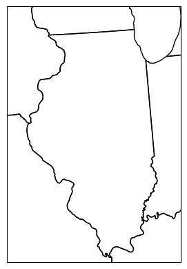
Your turn: Get into a small group and finish the map below by visualizing the buffer and identifying points within the buffer and points outside of the buffer (e.g., color coded, etc.).

import cartopy.crs as ccrs
import cartopy.feature as cfeature
import matplotlib.pyplot as plt

ax = plt.subplot(1, 1, 1, projection=ccrs.LambertConformal())
ax.set_extent([-92, -87, 37, 43])

ax.add_feature(cfeature.STATES)

<cartopy.mpl.feature_artist.FeatureArtist at 0x7a04a63e9280>

/usr/local/lib/python3.12/dist-packages/cartopy/io/__init__.py:242: DownloadWarning: Downloading: https://naturalearth.s3.amazonaws.com/10m_cultural/ne_10m_admin_1_states_provinces_lakes.zip
  warnings.warn(f'Downloading: {url}', DownloadWarning)

Chapter 7.3.2 -Choropleth Maps¶

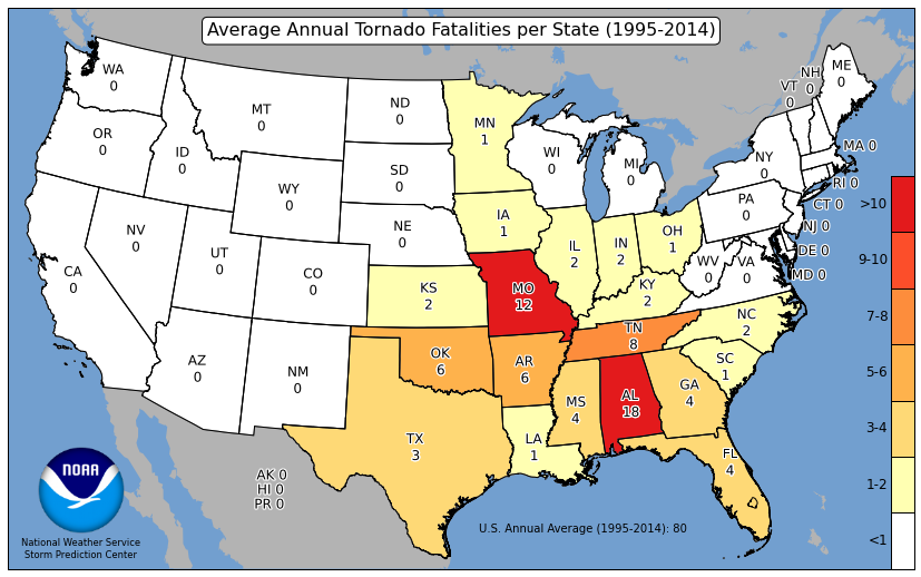
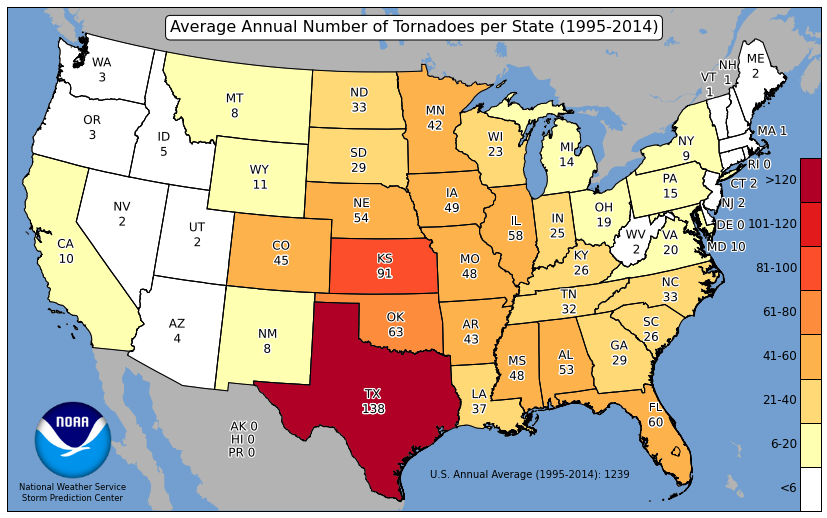
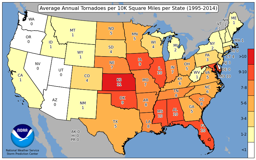
Choropleth maps are maps that can visualize relative frequencies of events within certain geometries. For example, the Storm Prediction Center has created maps that show the average count of tornadoes per state. The colormap helps the reader identify the relatively active states (deep red) with the less active states (white). This can be a more useful tool than just providing a table.

Spatial Join Applications

Choropleth maps require spatial joins to calculate the number of events within geometric bounds. In our case, we want to count the number of tornado reports that are within each state. This is just an extension of the problem above. We found that 110 tornadoes occurred within 40 km of NIU from 1950 - 2024 (75 years). We can then say that this region experiences about 1.5 tornadoes per year (110 tornadoes / 75 years = 1.47 t/yr), or 3 tornadoes every 2 years.

We first need to access the geometry of the states. We can easily do this through the cartopy interface. We can do some filtering to get to the CONUS. We also can see that the projection is lat/lon.

import cartopy.io.shapereader as shpreader

states_shp = shpreader.natural_earth(resolution='50m',
                                     category='cultural',
                                     name='admin_1_states_provinces')

states = gpd.read_file(states_shp)

# only USA
states = states[states.admin=="United States of America"]

# remove AK, HI, PR
states = states[~states.name.isin(['Alaska', "Hawaii", 'Puerto Rico'])]

print("states projection =", states.crs)
states.plot()

/usr/local/lib/python3.12/dist-packages/cartopy/io/__init__.py:242: DownloadWarning: Downloading: https://naturalearth.s3.amazonaws.com/50m_cultural/ne_50m_admin_1_states_provinces.zip
  warnings.warn(f'Downloading: {url}', DownloadWarning)

states projection = EPSG:4326

<Axes: >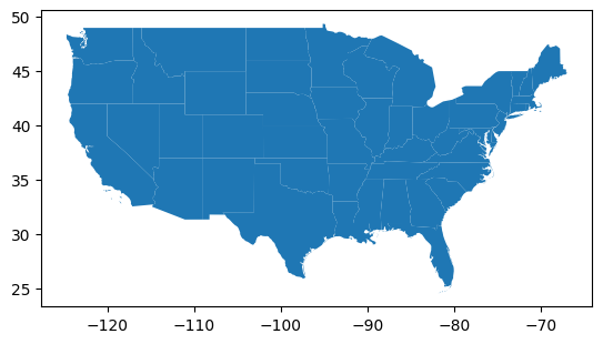

If we want to spatially join the US states with the tornado reports, we need to project these to albers:

states_aea = states.to_crs("EPSG:5070")

states_aea.plot()

<Axes: >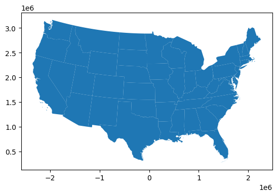

Next, we can try an left spatial join on the two datasets because most of the data will be matched (since most reports are in the CONUS) and we are just looking for counts.

NOTE: I have limited the columns for each dataset for illustrative purposes.

You can see that due to the left join and the position of the input GeoDataFrame, the geometry from the tornado reports are kept, but the state geometry is gone (think about this: how can you tell?).

The new columns, index_right and name, tell us to which polygon each report belongs.

choro = gpd.sjoin(
    tor_aea[['om', 'date', 'time', 'mag', 'geometry']],
    states_aea[['name', 'geometry']],
    how='left',
    predicate='within'
)

print("length of original dataset", len(tor_aea))
print("length of choro dataset", len(choro))
choro

length of original dataset 71813
length of choro dataset 71813

We can see repeats, which means that we can count the number of times each index_right shows up in the dataset using a groupby.size:

state_counts = choro.groupby('index_right').count()[['om']]
state_counts = state_counts.rename({'om': 'counts'}, axis=1)

state_counts

Now we can attach the counts using join. In this case, only one of the joined tables has geometry, so we want that table (states_aea) to be on the left side of the join method. The result is a new column named ‘counts’ attached to the right side of the states shapefile information. This retains all of the original states geometry.

states_aea_count = states_aea.join(state_counts)

# only show these columns for illustrative purposes
states_aea_count[['name', 'counts', 'geometry']]

We can now create an interactive choropleth map through Geopandas plotting interface and explore.

states_aea_count.explore(column='counts', popup=False, tooltip='counts')

Your Turn: Get into a small group and use the documentation of the explore function to customize a map that:

Has a title
Has a scale bar
Has a legend
Has a colormap similar to the map example
Only considers tornadoes between 1991 - 2020
Adjusts the counts for each state by the number of years to get a per-year count

If you complete that, make a map that adjusts the per-year counts by the area of the shape to get counts per year per 10,000 sq. miles.

If you complete that, make a map of fatalities per state. Note that you do not need a spatial join for this one, but you might need to change the approach.