L4 - Xarray

10 total points

Due: February 8th, 2026 at 11:59 p.m.

Directions:

1. Please rename the file by clicking on “LX-First-Last.ipynb” where X is the lab number, and replace First and Last with your first and last name.

2. Click File -> Save to make sure your most recent edits are saved.

3. In the upper right hand corner of the screen, click on “Share”. Click on “Restricted” and change it to “Anyone with the link”.

4. Copy the link and submit it on Blackboard. Make sure you follow these steps completely, or I will be unable to grade your work.

Overview¶

This lab will help you understand xarray and its capabilities. We will walk through some examples of how xarray can help solve Geoscience problems. Periodically, I will 1) ask you to either repeat the demonstrated code in a slightly different way; or 2) ask you to combine two or more techniques to solve a problem.

You can use generative AI to help answer these problems. The answer should still be in your own words. Think of the generative AI descriptions as those from a book. You still have to cite your source and you cannot plagiarize directly from the source. For every question that you used generative AI for help, please reference the generative AI you used and what your prompt or prompts were.

However, it is crucial that you understand the code well enough to effectively use generative AI tools that are likely to be widely available and recommended for use at many organizations. Although they are improving at an incredible rate, they still produce bugs, especially with domain-specific and complex problems. Make sure that you verify the answers before putting them in your own words.

Download¶

Make sure that you run the following commands to download the data used for this lab. This dataset includes all PRISM precipitation normals for each month.

%%bash uses Jupyter Magic Commands to process bash scripting code. This type of code is commonly used in linux-based systems to do basic file system tasks (renaming and/or moving files, setting up and executing scripts, etc.). In this case, the script loops through a set of numbers 1 - 12 to assist in automating the download and extraction of data used in this notebook.

You only need to run this once per session.

Install the required packages

Reading and Converting PRISM data¶

The PRISM data are originally in the geotiff raster data format. For this lab, we will use netCDF file format. Thus, we will convert the geotiffs to netCDF using the following code that loops through each month of precipitation data, renames some variables, and saves the file in netCDF format. This is not really that relevant to the lab, but I included it for completeness.

Reading in netCDF files with xarray¶

This lab will introduce you to how you can read and analyze netCDF files in the Geosciences.

The xarray package greatly simplifies the process of working with n-dimensional data. In other words, you will commonly interact with 3D (or even 4D) data in the Geosciences, and handling that with basic numpy methods can be tedious.

The most basic use of xarray is reading in a netCDF file. You can do it with the following code. Using the built-in display method can help you visually examine the data structure.

If you read data in for June, you will see the following:

• Dimensions: Dimensions are similar to indexes in numpy arrays, particularly n-dimensional numpy arrays.

• Coordinates: These define human-readable (usually) labels for dimension indexes. Coordinates include specific times, latitudes, longitudes, etc.

• Data variables: The actual Geoscience data at geographic positions defined by the coordinates. In this case, the dimensions of our Geoscience data are (time, lat, and lon). This is telling us that we could access precipitation data by indexing lat, lon, and/or time.

• Attributes: These are the “metadata” associated with the raw values and coordinates that give us more information about the data. This is a very convenient feature of netCDF data and is usually “packaged” with the data seamlessly.

We can quickly plot these data to see what they look like using the .plot.imshow() method. The squeeze() method is used to remove the single time dimension so you can plot the data on a 2D plot. This is the mean June accumulation of precipitation during the normal period.

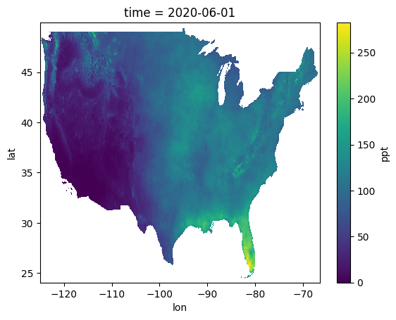
Problem 1¶

Run the following code and describe what each value means in your own words. Put your answer in this markdown:

Problem 2¶

There are two different ways to index data in the xarray dataset.

1. .sel(...): This requires selecting by the coordinate label. More similar to how data are accessed in pandas. If using float data, you need to include the argument method='nearest' because of floating point rounding and precision issues.

2. .isel(...): This requires selecting by the integer index. More similar to how data are accessed in numpy.

Interpret the output below in your own words. Specifically, explain (in this markdown) how two different indexing approaches got the same result?

Problem 3¶

All in the following code cell, open the netCDF file that represents January normals and set it equal to a variable named jan. Then, do the same for May (may). Find DeKalb’s lat/lon coordinates and use them with sel on both may and jan and print the value at that point. Convert it to inches. Does this make sense to you? What month has a higher normal precipitation amount for DeKalb? Answer in this markdown.

Problem 4¶

We will now explore the ability of xarray to work with 3-dimensional data. There is a file named monthly_normals_prism.nc that contains the combined values for each month in one file.

Notice when displaying the xarray dataset, the time dimension is now equal to 12. We can examine the coordinate values by printing out prism_all.time.

In your own words, explain “where” DeKalb’s normals for June exist in the 3D data structure from the perspective of:

1. prism_all.sel(..)

2. prism_all.isel(..)

Problem 5¶

xarray’s most useful methods include simple mathematical operations that we have used before with numpy: mean, sum, max, min, std, percentile/quantile. We can take advantage of the coordinates to transform our Geoscience expectations and best practices into simple method calls.

In your own words, explain the different results you see in the following code examples, including the size/shape of the resulting dimensions. How are they different from the original shape of (time: 12 lat: 621 lon: 1405). What would you call these results in more basic terms in your Geoscience area?

1. prism_all.mean()

2. prism_all.mean('time')

3. prism_all.mean(('lat', 'lon'))

Problem 6¶

Create a time series for DeKalb.

In xarray terms, a time series contains data from a coordinate that does not vary in space (a fixed location), but does vary in time.

Use it to complete the following line graph plot:

Problem 7¶

Create a Hovmoller diagram from prism_all to show how the precipitation totals along a line of longitude shift west and east from month to month.

In xarray terms, a Hovmoller replaces the lat (y) dimension with the time dimension, but keeps the lon (x) dimension. This is then plotted as a 2D image to examine how meteorological phenomena generally move over the course of a day or year in an east-west perspective.

Set the result to a variable named hov, use display to show its data structure, and use hov['ppt'].plot.imshow() to visually plot the result.

HINT: the final shape should be (time: 12 lon: 1405)

Problem 8¶

xarray can also group and resample like pandas.

We can use a combination of resample and mathematical methods to create meaningful Geoscience results.

In the case of prism_all, where there are 12 months of climate normal data, we might want to group months together into seasons.

We can use a special property of the time dimension when grouped in xarray: time.season. This converts all of the time data (in this case, the date of the start of each month) to group months together into:

1. DJF - Dec, Jan, Feb

2. MAM - Mar, Apr, May

3. JJA - Jun, Jul, Aug

4. SON - Sep, Oct, Nov

We can loop through the result to visualize the data structure of each group. In your own words, describe the shape of each seasonal result and your interpretation of each dimension. Place your answer in this markdown.

Problem 9¶

Explain the differences between the examples below in “general terms”.

1. prism_all.groupby('time.season').sum()

2. prism_all.groupby('time.season').mean()

3. prism_all.groupby('time.season').max()

In other words, what is this showing and what is the significance of these results in your Geoscience domain? What do you notice about the resulting dimensions and coordinates? How do the dimensions help you understand the result? Place your answer in this markdown.

Problem 10¶

Calculate the month with the highest precipitation total using prism_all and save the result in a variable named max_month. This should have the dimensions (lat: 621 lon: 1405) and should be plotted using max_month.plot.imshow