L2 - Geopandas

10 total points

Due: January 25th, 2026 at 11:59 p.m.

Directions:

1. Please rename the file by clicking on “LX-First-Last.ipynb” where X is the lab number, and replace First and Last with your first and last name.

2. Click File -> Save to make sure your most recent edits are saved.

3. In the upper right hand corner of the screen, click on “Share”. Click on “Restricted” and change it to “Anyone with the link”.

4. Copy the link and submit it on Blackboard. Make sure you follow these steps completely, or I will be unable to grade your work.

Overview¶

This lab will help you understand Geopandas and its capabilities. We will walk through some examples of how geopandas can help solve Geoscience problems. Periodically, I will 1) ask you to either repeat the demonstrated code in a slightly different way; or 2) ask you to combine two or more techniques to solve a problem.

Please do not use generative AI to answer these problems. In one example, I provide generative AI code that “solves” a problem and ask you to tell me where it went wrong. It is crucial that you understand the code well enough to effectively use generative AI tools that are likely to be widely available and recommended for use at many organizations. Although they are improving at an incredible rate, they still produce bugs, especially with domain-specific and complex problems.

Download¶

Make sure that you run the following commands to download the data used for this lab. This dataset includes all tornado warning and severe thunderstorm warning attribute, location, and metadata information for 2020 in the USA:

Install the required packages:

Geopandas can directly read shapefiles. To read in the data we just downloaded, run the following code:

Problem 1¶

You are tasked with visualizing the warning polygons associated with the derecho event of 2020 in Illinois. The first step is to subset the ~28,000 rows so that you are only working with data that overlaps your period of interest.

Use the .columns property to examine what columns are available for filtering purposes:

The ISSUED column is the time that the warning was first produced and sent by the local NWS station. We can examine just this column using column header indexing. We see that the date and time is formatted as such:

202005072219 -> YYYYMMDDHHmm

We could use string indexing to extract dates and times from this string, but it is easier just to turn it into a datetime object.

One way to do this is to use the pandas method to_datetime which can handle many datetime string formats withoput much effort. If you scroll all the way to the right below, you can see a new column named ISSUED_DT that contains a formated date:

This is very useful for us because we can access datetime methods by accessing the column via column indexing, accessing the dt (datetime) property for each row, and then access the properties: year, month, day, hour, minute, etc.

Below is an example of using this approach to print out all of the months for each row:

We can even do statistics on these properties. As we discussed in Chapter 6, value_counts is a very useful method that counts how often a unique value occurs (e.g., a month int) and then provides a sorted, descending list of the frequencies.

7 showed up the most (nearly 6000 times), which suggests that July was the most active month from a warning issuance perspective:

We can examine the breakdown of each type of warning throughout the year. We are most interested in:

1. SV (severe thunderstorm warning); and

2. TO (tornado warning):

Problem 1a¶

Use pandas filtering on the warning GeoDataFrame to compare monthly counts of tornado warnings and severe thunderstorm warnings.

Problem 1b¶

1. Use external sources to determine generally when the derecho moved through Illinois (date and hour range).

2. Use the image archive tool to examine radar loops from that time. If you correctly fill in the variables below, the resulting link should bring you to an animation on the Iowa State Mesonet page. NOTE: These are UTC times (add 5 hours to central time in August).

Problem 1c¶

Based on you manual assessment of the radar animation, use ISSUED_DT to filter warnings for rows that are within the time range of the derecho passing through Illinois and are tornado or severe thunderstorm warnings. Set the result to a new variable named warn_derecho.

datetime.datetime takes the arguments year, month, day, hour, and minute in order.

Problem 1d¶

Verify that your date range is correct by printing out the max and min times within the subset’s ISSUED_DT.

Why might these not match the bounds you specified above (ANSWER IN MARKDOWN)?

Answer:

Problem 2¶

Considering your map project is an important part of any analysis that includes spatial data types. We can examine the projection information associated with the shapefile we read in earlier by using the crs property:

The coordinate system and mapping information associated with the warnings is the basic “latitude / longitude”. This is very convenient for sharing data and long-term file storage, but it can cause inconsistencies in your analysis.

For example, let’s look at the area of the qualifying warnings by using the area property in the GeoDataFrame. This is based on the shapely property that is built-in to spatial data types that have areas (e.g., polygons, etc.).

You will notice that you have a warning that tells you, basically, to not trust the area that is returned! These areas are very small because they are “square degrees”.

geopandas also has a solution to this issue. There is a method called to_crs that will automatically convert your geometry between coordinate systems.

The easiest way to perform this task is to find an appropriate projection code. This website is useful for getting many of the most common, non-custom, projection codes: https://epsg.io/

Typically, if we are trying to calculate area, we want what is called an “equal area” projection. For the US, there are two popular choices:

1. USGS Contiguous USA Albers Equal Area (EPSG:5070; units = meters)

2. UTM 16 N (if examining Illinois or states directly North or South; EPSG:26916; units = meters)

A “USA Albers Equal Area” is a good general use projection for the USA. UTM 16 N is only good for specific states, however, it is more accurate than the general USA equal area (2.0 m accuracy).

Let’s choose the USA version and perform the projection below.

NOTE: this will have no impact on your attribute columns, just the geometry columns and the spatial properties of the GeoDataFrame.

Problem 2a¶

Compare the area differences in sq. km between albers and UTM by projecting to UTM and creating a new column. Display both columns as demonstrated above.

Problem 2b¶

Find the mean size (in sq. km) of the warnings during the period you are examining. What is the size of DeKalb County? Do your results make sense?

Problem 2c¶

Compare the mean size of tornado warnings and severe thunderstorm warnings. Which are bigger on average?

Problem 2d¶

Run another area analysis that you find interesting or are curious about. Explain your approach in the markdown and interpret the results.

Problem 3¶

Plotting geometry on a cartopy map is relatively straightforward. The only tricky part can be handling projections.

For simplicity, we are going to use the filtered but lat/lon version of the GeoDataFrame warn_derecho.

We will use cartopy to map the warning data.

Making a simple cartopy map only takes a few lines of code. We will talk more about mapping in future labs, but here are the basics:

import cartopy.crs as ccrs: ccrs handles all of the projection duties

import cartopy.feature as cfeature: cfeature handles convenient methods to plot common boundaries (US States, etc.).

These two imports will be included in most, if not all, of your code that involves cartopy mapping.

The code below:

1. Sets the map projection to lat/lon (projection=ccrs.PlateCarree())

2. Adds US states to the map ax.add_feature(cfeature.STATES)

3. Sets the map extent to areas centered on Illinois.

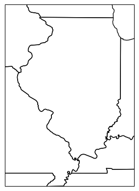
Problem 3a¶

The add_geometries method can add any geometry with geographic information to the map. This function takes a list or numpy array of geometries. Create a polygon that would be within Illinois based on its lat/lon coordinates.

Problem 3b¶

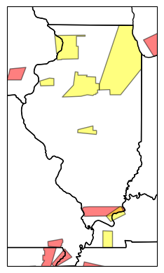
Remove two instances of .sample(100) from the code below once you determine the correct subset for warn_derecho in Problem 1c.

Modify the following code so the tornado warnings are red and severe thunderstorm warnings are yellow in your 2020 derecho subset.