L7 - Scikit-Learn - Decision Trees¶

Directions:

1. Please rename the file by clicking on “LX-First-Last.ipynb” where X is the lab number, and replace First and Last with your first and last name.

2. Click File -> Save to make sure your most recent edits are saved.

3. In the upper right hand corner of the screen, click on “Share”. Click on “Restricted” and change it to “Anyone with the link”. Make sure you also share it with ahaberlie1@gmail.com.

4. Copy the link and submit it on Blackboard. Make sure you follow these steps completely, or I will be unable to grade your work.

Overview¶

This lab will help you understand scikit-learn and its decision tree capabilities. We will walk through some examples of how scikit-learn can help solve Geoscience problems. Periodically, I will 1) ask you to either repeat the demonstrated code in a slightly different way; or 2) ask you to combine two or more techniques to solve a problem.

You can use generative AI to help answer these problems. The answer should still be in your own words. Think of the generative AI descriptions as those from a book. You still have to cite your source and you cannot plagiarize directly from the source. For every question that you used generative AI for help, please reference the generative AI you used and what your prompt or prompts were.

However, it is crucial that you understand the code well enough to effectively use generative AI tools that are likely to be widely available and recommended for use at many organizations. Although they are improving at an incredible rate, they still produce bugs, especially with domain-specific and complex problems. Make sure that you verify the answers before putting them in your own words.

Model performance assessment

When assessing model performance, we typically separate the sample data into three subsets. Think of your own experiences preparing for an exam as motivation for the subsets:

1. Training data - this is what the machine learning approach uses to generate a model. Similar to lectures/homework/assignments/etc. in class.

2. Validation data - this is what is used to do quick “spot checks” on the model and help determine optimal model settings. This is similar to doing a practice quiz and learning what you need to focus on before the exam.

3. Testing data - this is what is used to test the performance of the model. This is similar to finally taking the exam.

I have provided you with the training and testing datasets. We will also generate the validation dataset below:

Problem 1¶

Answer in the markdown: Assess the following decision tree in your own words. What is the performance of this tree? What are some caveats associated with this performance?

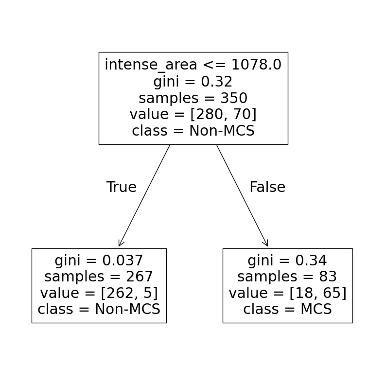
Problem 2¶

Answer in the markdown: Using the validation dataset, the following example shows two possible decision tree configurations and the F-score for each case. In your own words, assess the performance of each case and identify which case you should choose. What is the difference between the two trees?

Problem 3¶

Answer in the markdown: Using the validation dataset, the following example shows two possible decision tree configurations and the F-score for each case. In your own words, assess the performance of each case and identify which case you should choose. What is the difference between the two trees?

Problem 4¶

Automated model selection

sklearn has an automated way to test out many different model configurations: GridSearchCV. This class requires you to think about the following options:

1. estimator: this is your untrained DecisionTreeClassifier instance. Do not run fit.

2. param_grid: this is a dictionary with the parameter names and all the possible values you want to test with that parameter.

3. scoring: this defines how GridSearchCV will determine the “best performing” model on validation data.

4. cv: this is how you will separate the training and validation data. In some cases, it might be appropriate to have sklearn handle this with an approach that randomly removes 10% of the data in k different ways. In our case, we will use a predefined split, since it is important to examine “new” data that has temporal independence.

This approach essentially recreates the loops we did in the previous problems. You just have to define the possible values for each parameter.

The first step is to look up the documentation for the model you are using. We are using a DecisionTreeClassifier. On that page you will see Parameters along with several different names of parameters and descriptions. You can try different ranges of numbers that make sense for each parameter. These need to be put in a dictionary.

For this case, we will test the following values to see which combination works best:

1. test criterion of gini (we calculated this earlier) or entropy

2. test max_depth of None (no limit), 2, 4, 6, 8, and 12

3. test min_samples_split of 2, 5, 10, and 20

4. test min_samples_leaf of 1, 2, 5, and 10

We can use ParameterGrid to see all the different combinations.

Answer in the markdown in your own words:

Why are there 192 rows?

Give an example of manually creating a DecisionTreeClassifier model based on the parameters in row 50 (index 49).

Next, we will define the split used to decide what data are supplied to the training process and what data are supplied for the validation process. Since we already have those subsets, we will use the PredefinedSplit approach.

The model selection approach, by default, assumes that we have one subset of feature vector information (i.e., train_x and val_x) as well as one subset of label information (i.e., train_y and val_y).

The best way to combine these two subsets is to use concatenate from numpy. We will use this to “attach” val on to the end of train. As long as we know where this happens, it is easy to define how to tell the model selection step how to split the data.

First, here is a smaller example:

trainx is an ndarray of 2 feature vectors with 3 features and trainy is a ndarray of 2 labels associated with those feature vectors. Similarly, valx and valy are the same, except for one sample.

When you run the concatenate method, you see the result is just a combination of the train and val subsets.

If you wanted to tell the model selection approach that these indices were train with a value of -1 (not in the ‘val’ set) and val with a value of 0 (in the val set), you would define split as you do below. The model selection approach will keep all indices of 0 off to the side and use all indices of -1 to train each model variant. Each model variant will tested with the 0 indices (the validation data), and the best performing model on those data will be selected.

Here is the full concatenation:

We know that the train_x data end at index len(train_x), so we can easily create the -1 and 0 arrays using a number of approaches, for example:

We then pass this array into PredefinedSplit

Finally, we build a basic DecisionTreeClassifier and pass the required information into GridSearchCV. The new code here is:

1. make_scorer: a wrapper around the f1_score we used before.

2. refit: if True, retrain the best performing model and provide it as best_estimator_.

Problem 5¶

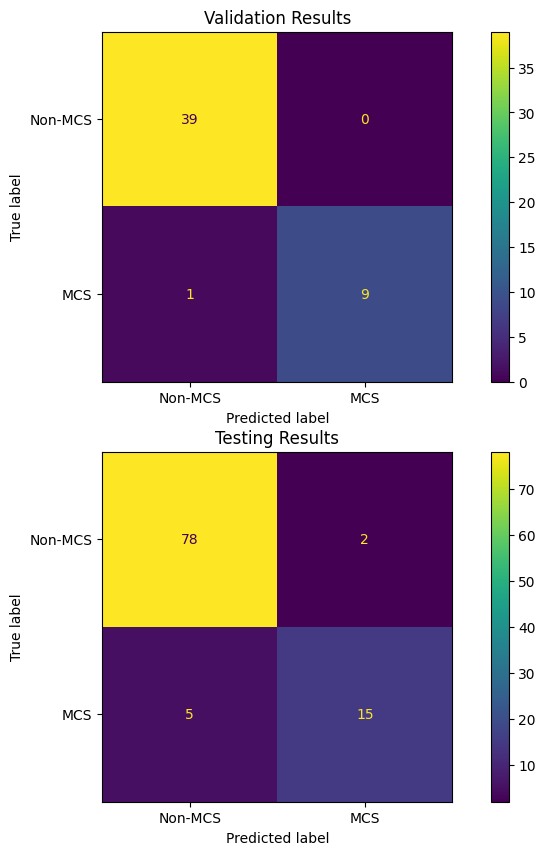
Now, compare the results on the validation data to those on the testing data.

Calculate TP, FP, FN, TN, recall and precision for both testing/validation using the plots below (confusion matrix). Verify that the F score is correct.

Answer in the markdown: Do the validation data results match with the testing data? Why or why not? What do you think this suggests about the ability of the model to generalize to new, unseen years?